- Startpagina tijdschrift
- Volume 22 (2018)
- Numéro 3
- Forest mapping and species composition using supervised per pixel classification of Sentinel-2 imagery
Weergave(s): 0 (0 ULiège)
Download(s): 0 (0 ULiège)
Forest mapping and species composition using supervised per pixel classification of Sentinel-2 imagery

Nota's van de redactie
Received 20 December 2017, accepted 20 June 2018, available online 6 Augut 2018
This article is distributed under the terms and conditions of the CC-BY License (http://creativecommons.org/licenses/by/4.0)
Résumé
Cartographie forestière et composition spécifique par classification supervisée par pixel d’imagerie Sentinel-2
Description du sujet. Étudier l’état et l’évolution des forêts est essentiel pour assurer une gestion durable maintenant leurs fonctions écologiques et socio-économiques. La télédétection est un outil précieux pour le développement de ces connaissances.
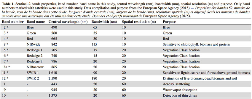
Objectifs. Cette étude analyse l’opportunité offerte par l’imagerie Sentinel-2 (S2) pour cartographier les forêts de l’écorégion de l’Ardenne belge. Le premier objectif de classification était la création d’une carte forestière à l’échelle régionale. Le second objectif était la discrimination de 11 classes forestières (Fagus sylvatica L., Betula sp., Quercus sp., other broad-leaved stands, Pseudotsuga menziesii (Mirb.) Franco, Larix sp., Pinus sylvestris L., Picea abies (L.) H.Karst., young needle-leaved stands, other needle-leaved stands, and recent clear-cuts).
Méthode. Deux scènes S2 ont été utilisées et une série d’indices spectraux ont été générés pour chacune d’entre elles. Nous avons réalisé une classification supervisée par pixel avec l’algorithme de classification Random Forest. Les modèles de classification ont été générés avec un jeu de données S2 pur et avec des données 3D supplémentaires pour comparer les précisions obtenues.
Résultats. Les données 3D ont légèrement amélioré la précision de chaque objectif, mais l’amélioration globale de précision fut uniquement significative pour l’objectif 1. La carte forestière produite avait une précision globale de 93,3 %. Le modèle testant la discrimination des espèces d’arbre fut encourageant également, avec une précision globale de 88,9 %.
Conclusions. Tenant compte des simples analyses réalisées dans cette étude, les résultats doivent être interprétés avec prudence. Cependant, ce travail confirme le grand potentiel de l’imagerie S2, particulièrement les bandes SWIR et red-edge, qui jouèrent un rôle essentiel dans ce travail.
Abstract
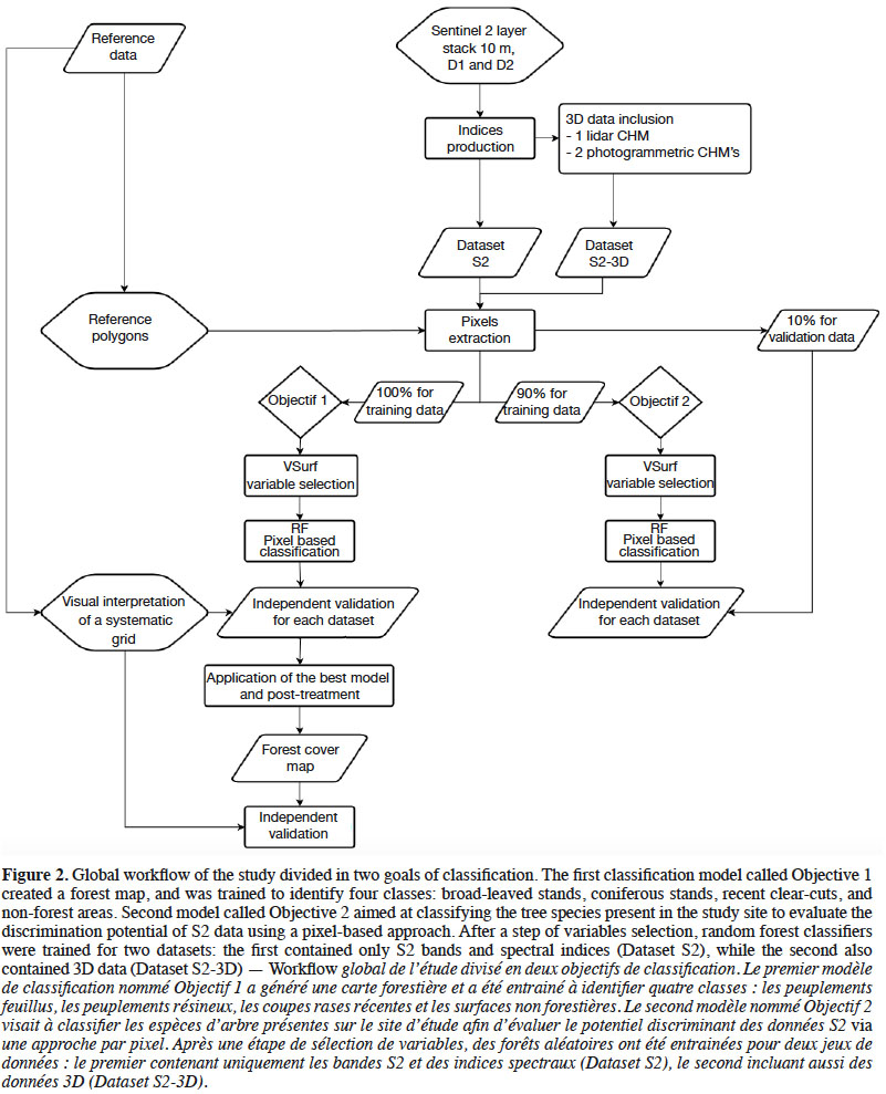
Description of the subject. Understanding the current situation and evolution of forests is essential for a sustainable management plan that maintains forests’ ecological and socio-economic functions. Remote sensing is a helpful tool in developing this knowledge.
Objectives. This paper investigates the new opportunities offered by using Sentinel-2 (S2) imagery for forest mapping in Belgian Ardenne ecoregion. The first classification objective was to create a forest map at the regional scale. The second objective was the discrimination of 11 forest classes (Fagus sylvatica L., Betula sp., Quercus sp., other broad-leaved stands, Pseudotsuga menziesii (Mirb.) Franco, Larix sp., Pinus sylvestris L., Picea abies (L.) H.Karst., young needle-leaved stands, other needle-leaved stands, and recent clear-cuts).
Method. Two S2 scenes were used and a series of spectral indices were computed for each. We applied supervised pixel-based classifications with a Random Forest classifier. The classification models were processed with a pure S2 dataset and with additional 3D data to compare obtained precisions.
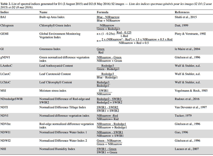
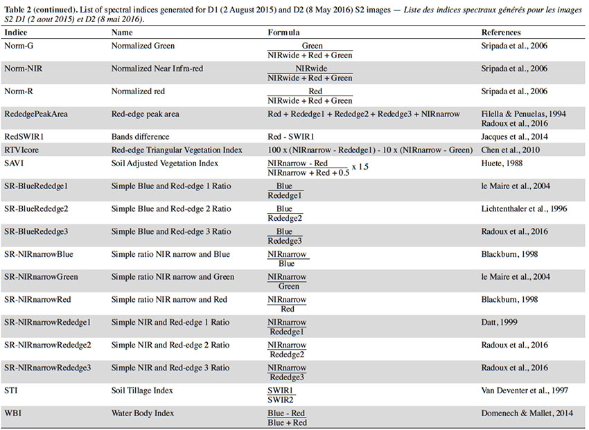
Results. 3D data slightly improved the precision of each objective, but the overall improvement in accuracy was only significant for objective 1. The produced forest map had an overall accuracy of 93.3%. However, the model testing tree species discrimination was also encouraging, with an overall accuracy of 88.9%.
Conclusions. Because of the simple analyses done in this study, results need to be interpreted with caution. However, this paper confirms the great potential of S2 imagery, particularly SWIR and red-edge bands, which are the most important S2 bands in our study.
Inhoudstafel
1. Introduction
1Forest ecosystems provide important services to society, and sustainable management and adapted policies are essential to maintain their ecological and socio-economic functions. Forest managers and policy makers must consider the relationships between forest function and ecosystem characteristics and the evolution of forests in order to manage forests and make regional decisions (Führer, 2000; Lindenmayer et al., 2000). Given the globalization of today’s society, this need has become even more important, as understanding forests is important for international agreements and reporting requirements (e.g. the Kyoto Protocol).
2For decades, field inventories have been used to better characterize forest. National inventories exist in countries around the world and have evolved over time to adapt to users’ needs (Tomppo et al., 2010). Field inventories provide timely and accurate estimates of forest resources and their evolution at a large scale. Nevertheless, this method is time-consuming and quite expensive. Furthermore, an inventory of an entire area is, for obvious reasons, impossible and sample-based procedures are necessary. Therefore, technological innovation is becoming crucial to improve the efficiency of measurements and estimations while making the production of inventory data simpler (McRoberts & Tomppo, 2007).
3Remote sensing is one of the technological tools at our disposal: it decreases the cost of data acquisition, increases the area it is possible to cover without sampling, and enables the production of high-resolution forest attribute maps. Remote sensing enables the production of map layers that give precious information about the distribution of forest resources. These complement sample-based procedures in the field and today are commonly used by researchers and managers (McDermid et al., 2009).
4Today advances in technology such as satellite remote sensing and digital photogrammetry have increased the possible applications of remote sensing and image classification. Light detection and ranging (LiDAR) data and photogrammetry technologies have made it possible to use 3D data, such as Canopy Height Models (CHM) when investigating forests. These technologies improve the classification accuracy of forest classes (Waser et al., 2011). However, 3D data is still rare at the large scale and the technology remains expensive.
5This may be different for satellite imagery. On 28 February 2008, the European Union (EU) and European Space Agency (ESA) signed an agreement over the creation of the COPERNICUS program. The aim of this program is to provide earth surface monitoring services (European Commission, 2015) (Land, Atmosphere & Marine Monitoring, Climate Change, Security & Emergency Management Services). The launch of the two Sentinel-2 (S2) satellites is an opportunity to enhance forest characterization on a large scale. The satellites multispectral 13-band sensors produce high-quality images at a 5-day equatorial temporal resolution (Suhet & Hoersch, 2015). Such an availability of free data is unprecedented and will substantially promote research in this topic.
6In preparation for the arrival of the new S2 imagery, Inglada et al. (2017) present a methodology to automatize the production of a land cover map at the country scale using high-resolution optical image time series. Using this methodology, the study constructs a map of metropolitan France with a coefficient of kappa 0.86 describing 17 land cover classes, including broad-leaved forest and coniferous forest. In the first study to use pre-operational S2 data, Immitzer et al. (2016) test both a pixel-and object-based classification of tree species in Germany for 7 classes, getting an overall accuracy (OA) of 0.64 and 0.66, respectively. These studies demonstrate the powerful potential of satellite imagery for forest mapping, and research is necessary to exploit the potential of these new S2 data. In their review of tree species classification studies, Fassnacht et al. (2016) observe the increasing number of works on this topic over the last 40 years. However, they note that most investigations are oriented toward optimizing classification accuracy over a relatively small test site and it is therefore often difficult to draw general conclusions from these studies. The authors recommend using well-defined applications in future research in order to avoid purely data-driven studies of limited values and increase understanding of broader factors affecting tree species classification.
7In this context, we use S2 imagery to investigate image classification in European temperate forests at the regional scale. Our study has three goals:
8– to create a highly accurate regional forest map using S2 imagery;
9– to evaluate the potential of S2 imagery in identifying the main tree species encountered in the study area;
10– to assess the benefits of incorporating 3D data into our study of the previous two goals and therefore determining how precise S2 data is in these approaches.
11For these purposes, we implemented supervised classification per pixel using a random forest (RF) algorithm. We used two S2 images acquired at different dates to take account for species seasonality. Then, we computed a range of spectral indices. After a step of variables selection, we trained random forest classifiers for two datasets: the first contains only S2 bands and spectral indices, while the second also contains 3D data. The quality of the results was assessed and compared in terms of a confusion matrix with a strong reference dataset.
2. Materials
2.1. Study site
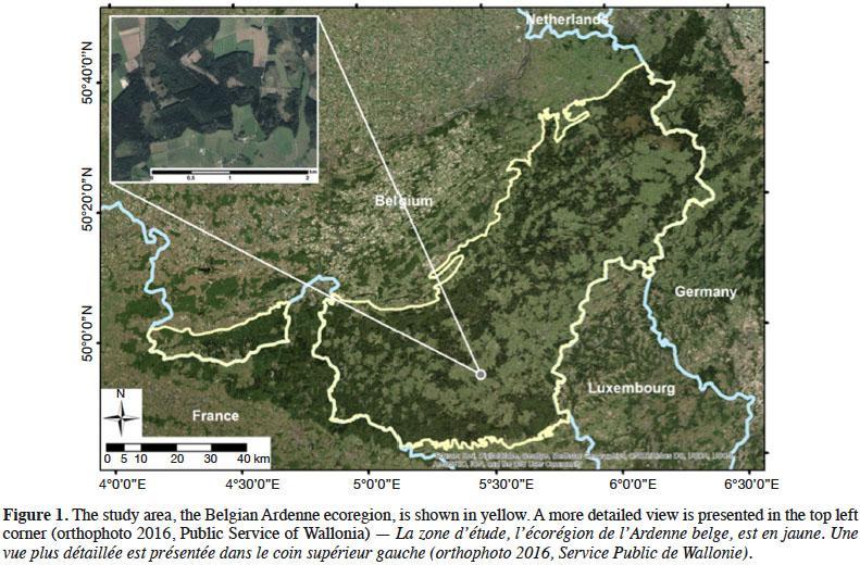
12The study was conducted for the entire Belgian Ardenne ecoregion. This region constitutes a plateau whose altitude increases gradually from the South-West to the North-East, culminating at nearly 700 m. The annual mean temperature is smaller than 9 °C and annual precipitations are nearly 1,200 mm. With an afforestation rate of 58%, the Ardenne represents 333,850 ha of forest and is the largest forest area in Wallonia. This forest is mainly coniferous (64%), according to Wallonia’s Regional Forest Inventory (RFI) (Alderweireld et al., 2015), and the most frequently found tree species are (in order of quantity): spruce (Picea abies [L.] H.Karst.), oak (Quercus sp.), beech (Fagus sylvatica L.), Douglas fir (Pseudotsuga menziesii (Mirb.) Franco), pine (Pinus sp.), and larch (Larix sp.). These six species represent 85.8 % of the forest. Most of the time, coniferous stands are pure species plantations. Deciduous stands are most of the time naturally regenerated and thus present an uneven-aged structure and a composition dominated by beech and oak, the level of mixture being driven mainly by soil depth and topography. Figure 1 provides an overview of the study site.
2.2. Remotely sensed data
13Sentinel-2. The onboard S2 sensor is a passive multi-spectral instrument (MSI). It provides 13 spectral bands (Table 1). In order to simplify pre-processing, the only two available S2 images with less than 10% cloud cover over the entire Ardenne ecoregion were selected. Their sensing times were 2 August 2015 and 8 May 2016 (further referred as D1 and D2). These dates have a potential interest as they could help to difference some broad-leaved species between themselves or from resinous species. Indeed in this region, in May, Fagus sylvatica and Betula sp. have begun foliation period since more than a month while Quercus sp. have just started (https://fichierecologique.be). It is widely acknowledged that reflectance from the Earth’s surface, called top-of-atmosphere (TOA), is significantly modified by the atmosphere (Jensen, 2005; Lillesand et al., 2008; Richards, 2013). There are many remote sensing studies that have investigated how to reduce the effects of the atmosphere on the signal (Kaufman et al., 1997; Song et al., 2001; Guanter et al., 2008). This is even more important in case of multi-temporal date analyses (Agapiou et al., 2011; Hagolle et al., 2015), therefore we used the atmospheric correction proposed by the Sen2Cor processor (version 2.2.) (Müller-Wilm, 2016). Hence, Level-1C data were processed into Level-2A (bottom-of-atmosphere corrected reflectance images). S2 bands at 20 m of spatial resolution were resampled at 10 m during this step (nearest neighbor method). Then we compiled a layer stack of 20 spectral bands with D1 and D2.
143D data. Three Canopy Height Models (CHM) and one slope layer, based on LiDAR and photogrammetric point clouds, were used covering the entire study area at a resolution of 1 m.
15A CHM was made using LiDAR (LiDAR DSM - LiDAR DTM) and referred to as CHM3 in this paper. The average point density of small footprint discrete airborne Lidar data was 0.8 points·m-1. Survey flights were realized by the Public Service of Wallonia from 12 December 2012 to 21 April 2013 and from 20 December 2013 to 9 March 2014. The survey covered Wallonia with a regional digital terrain model (1 m ground sampling distance [GSD]). A digital surface model (DSM) at the same resolution was also computed and a slope layer was generated based on the Lidar digital terrain model (DTM).
16For two other CHMs, raw images from two regional orthophoto datasets (acquired by the Public Service of Wallonia) were used to generate two high-density photogrammetric point clouds. Both survey flights took place between April and September, the first in 2006 and 2007 (0.50 m GSD), the second in 2009 and 2010 (0.25 m GSD). Considering that the regional topography did not change significantly, hybrid CHMs were computed using photogrammetric DSM and LiDAR DTM, as described above, following the approach of Michez et al. (2017) (photogrammetric DSM-LiDAR DTM). Their spatial resolution is 1 m. The precision of this approach has been evaluated in Michez et al. (2017) using field tree height measurements (root mean square error smaller than 3 m). These hybrids CHM are called CHM1 and CHM2 in this paper. They were used in this study to improve the detection of recent clear cuts and young stands, adding height information in the past.
17These four layers (CHM1, CHM2, CHM3, and SLOPE) were aggregated at 10 m of spatial resolution using median value.
3. Methods
3.1. Image classification models
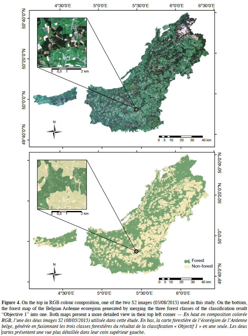
18To accomplish our first two goals, we defined two models of classification. The model called Objective 1 created a forest map, and was trained to identify four classes: broad-leaved stands, coniferous stands, recent clear-cuts, and non-forest areas. The non-forest class dataset contained an equal proportion of observations for agricultural lands, urban landscapes, and water bodies. In order to create our forest map, we applied the obtained classifier to the entire study area. We then generated a forest land use map by merging the three forest classes into one. By first growing a model with four classes, clear cuts are integrated into the produced forest map, as it forms an integral part of the forest estate covered by management plans.
19Second model called Objective 2 aims at classifying the tree species present in the study site to evaluate the discrimination potential of S2 data using a pixel-based approach. Based on the RFI, we defined 11 classes that corresponds to the main species or types of stands: beech, birch (Betula sp.), oak, other broad-leaved stands (OB), Douglas fir, larch, Scots pine (Pinus sylvestris L.), spruce, young needle-leaved stands (YN), other needle-leaved stands (ON), and recent clear-cuts (RCC). Young stands correspond to plantations between 4 and 12 years old, and recent clear-cuts are stands that have been harvested in the last four years. For each class, pixels contain at least 80% of the species or group of species.
20The global workflow of the study is synthesized in figure 2.
3.2. Dataset preparation
21In order to determine the most pertinent classification variables in each model, we added a large selection of spectral indices to the original S2 dataset. Each indice was generated for D1 and D2. The list is presented in table 2.
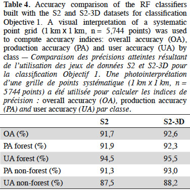
22We then created another dataset that include 3D data and compared results of the two datasets for each classification objective. In other words, for each objective we tested the following datasets: the S2 bottom-of-atmosphere data D1 and D2 with spectral indices (S2) and the S2 bottom-of-atmosphere data D1 and D2 with spectral indices and 3D data (S2-3D).
23All together, there were 10 S2 Bands, 34 indices by sensing time, 3 CHM dates, and 1 slope layer. So, depending on whether we included 3D data, we had 89 or 93 variables by dataset.
24Reference pixels were produced from delineated management forest units (DFU) extracted from the regional forest administration geodatabase and from four bands (RGB and IR) 0.25 m resolution orthophotos covering the entire region. These image layers are available for the years 2006, 2009, 2012, and 2015 (http://geoportail.wallonie.be).
25DFU were used for both Objectives 1 and 2 to extract reference data for forest classes. Before that, DFU polygons were visually interpreted to verify eventual errors or modifications since the last update. For each class, the chosen forest stands were supposed to be “pure stands” according to the DFU database (percentage > 80%). Table 3 shows by class the number of polygons and the number of extracted pixels. Reference polygons were delineated for non-forest classes by visual interpretation of orthophotos.

3.3. Variable selection and classification
26The following steps were executed in the same way for Objectives 1 and 2 using Dataset 1 or 2 (Figure 2). Before building classification models, we rationally reduced the number of variables by selecting the most important using VSurf (Genuer et al., 2016) in R software (R Core Team, 2016). The VSurf package allows variable selection based on the estimation of RF’s variable importance (Genuer et al., 2015). As a result, the process provides two variables subsets. The first, called “variable interpretation”, is intended to show variables highly related to the response variable. It does not matter if there is some, or even much, redundancy in this subset. The second, called “prediction”, is a smaller subset with low redundancy intended to assure a good prediction of the response variable.
27The following parameters were set to allow the maximum performance in a reasonable time with the used computer:
28– each RF was built using ntree = 1,000 trees, the number of variables randomly sampled as candidates at each split (mtry) was set by default (sqrt[p], where p is the number of variables);
29– the number of random forests grown was 20 for the three main steps of the Vsurf process: “thresholding step”, “interpretation step”, and “prediction step” (nfor.thres = 20, nfor.interp = 20 and nfor.pred = 20);
30– the mean jump is the threshold of decreasing mean OOB error used in the Vsurf’s prediction step to add variables to the model in a stepwise manner. It was multiplied 4 times (nmj = 4) in order to make this step more selective, considering the large number of variables.
31For the two objectives, we realized supervised classifications per pixel with a RF classifier (Breiman, 2001), using the randomForest package (Liaw & Wiener, 2002) in R software (R Core Team, 2016). Only the variables selected during the prediction step of VSurf were considered for this classification. The process was executed with 2,000 trees to grow and mtry set by default. A series of parameters combinations were tested to find the most relevant parameters for this study. Before training the models, the number of observations by class was randomly downsampled to balance classes.
3.4. Accuracy assessment
32All the reference data extracted from DFU polygons were used to train Objective 1. The accuracy assessment was carried out with a set of points systematically distributed over the study area (1 km x 1 km, n = 5,744 points) and photo-interpreted on the orthophotos. Confusion matrices were built comparing attributed classes for these points.
33Concerning Objective 2, 10% of the reference data extracted from DFU polygons was randomly selected to create a validation dataset. The number of observations by class was randomly downsampled to balance classes for the validation. Confusion matrices were built using these validation data. For Objectives 1 and 2, we computed the OA (overall accuracy) as well as producer (PA) and user accuracy (UA) for each class.
4. Results
4.1. Objective 1: forest map
34Comparing the performance of both datasets. Table 4 shows the accuracy of the forest maps generated using the S2 and S2-3D datasets. These results were computed before post treatments and are presented to compare dataset performances. The presentation of the final forest map is described in Section 4.1.3. S2-3D gave the best results, with an overall accuracy difference of 0.9% between the two approaches. This difference is significant (p-value = 0.002421, McNemar’s chi-squared test realized on the contingency table of correctly classified and incorrectly classified points). The PA of the non-forest class had the highest difference in accuracy (1.7%) between S2 and S2-3D. The lowest difference in accuracy (0.4%) was for the PA of the forest class.
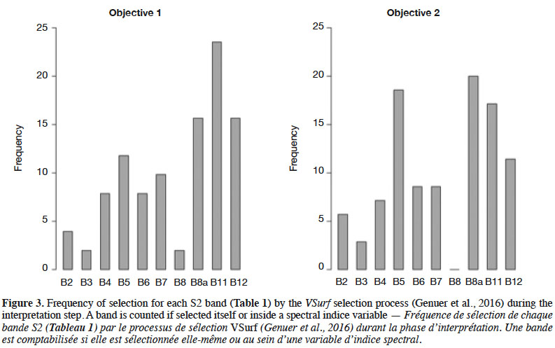
35Selected variables. The results presented in this section are based on the classifier trained with the S2-3D dataset, which obtained the best precisions. Figure 3 illustrates which S2 bands were mostly identified as relevant regarding our classification goals. A band was counted if it was selected at the VSurf interpretation step and each time it was used in a variable selected during the interpretation step. For Model 1, the three bands used the most were B8A, B11 and B12, all of which have a 20 m GSD.
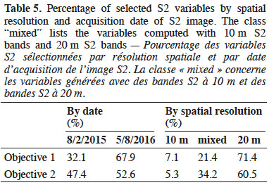
36In table 5, variables were sorted according to their sensing date and native spatial resolution. The term “mixed” means that S2 bands of both spatial resolutions were used to generate the index.
37Fourteen variables were selected during the VSurf prediction step. The list is presented in descending order of occurrence: CHM2, CHM3, B11-D2, CHM1, B7-D2, B12-D1, SLOPE, STI-D1, NDTI-D1, RTVIcore-D2, B5-D2, MSI-D2, NDrededgeSWIR-D1, and B5-D1.
38Production of a forest map. The RF classifier generated with previous variables was used to compute a final forest map. This map was then filtered using the Majority Filter tool of ArcMap® (Number of neighbors to use: 8, Replacement threshold: MAJORITY). Figure 4 presents the result. A validation was carried out for the produced map. The OA value of the confusion matrix was 93.3%. PA and UA were 93.2% and 95.8% for the forest class while it was 93.3% and 89.5% for the non-forest class.
4.2. Objective 2: tree species classification
39Comparing the performance of both datasets. In order to compare the accuracies of achieved results for both the S2 and S2-3D dataset, user accuracies of all classes have been summarized by mean to make the comparison easier. For dataset S2, OA and the user accuracy mean (UA mean) were 88.5% and 88.6% while for dataset S2-3D, it was 88.9% and 89%. As with Model 1, the 3D dataset gave the best results but the differences in precision can be considered as negligible: in all cases the value was less than 0.5%.
40Selected variables. The results presented in this section concern the classifier trained with the S2-3D dataset that obtained the best precision values. They are summarized in figure 3 and table 5. The three most-selected bands at the VSurf interpretation step were B8A (NIR narrow), B5 (Red Edge 1), and B11 (SWIR 1), all of which have a 20 m GSD.
41Eighteen variables were selected during VSurf prediction step. The list is presented in descending number of appearances: SLOPE, CHM1, CHM2, CHM3, RedSWIR1-D2, B8A-D2, B7-D2, B11-D2, NDrededgeSWIR-D1, B5D2, MSI-D2, NDWI1-D2, B12-D2, B6-D2, B11-D1, STI-D1, B5-D1, and LChloC-D1.
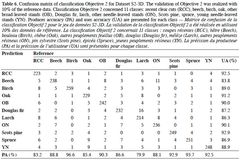
42Accuracy of the best classifier. Achieved accuracies with the S2-3D dataset are presented in detail by a confusion matrix (Table 6). The OA was 88.9%. The worse PA concerned the larch (79.9%) and recent clear cut (83.2%) classes. The worst UA were for beech (83.8%) and larch (86.3%).
5. Discussion
5.1. Variable selection
43It is interesting to observe the difference between Objectives 1 and 2 in figure 3. In Objective 1, the most selected bands were found, in order of number of appearances, B11, B8a, and B12. In Objective 2 the most selected bands were B8a, B5, and B11. These results are in line with the goals of classification models and band properties. Indeed, Objective 1 aimed at distinguishing forest classes (coniferous stands, broad-leaved stands, and recent clear-cuts) from non-forest areas. The second classification objective was separating tree species classes present on the study site. B11 is sensitive to forest above ground biomass and B12 facilitates distinction of live biomass, dead biomass, and soil (Table 2), thus B11 and B12 have more importance in Objective 1 where there are non-forest classes. B5 and B8a are more related to Objective 2; indeed, vegetation classification is the only goal in this case. Figure 3 shows the importance of shortwave infrared (SWIR) (B11 and B12) and the red-edge band B5 for both models, as mentioned in other studies (Schuster et al., 2012; Fassnacht et al., 2016; Immitzer et al., 2016; Radoux et al., 2016).
44Looking at table 5, we can see that the most selected variables have a GSD of 20 m. As a consequence, the resolution of the resulting maps was not really 10 m; even more without the use of 3D data. This confirms the relevance of spectral bands sensed by S2 but reminds us that spectral resolution can be more important than spatial resolution for vegetation discrimination at a regional scale.
45Selected variables were well distributed between the two S2 images taken on different dates, especially for Objective 2. It appears that image interaction was useful. Choosing the time of image acquisition in relation to species’ phenological cycle is a possible way to improve discrimination. Immitzer et al. (2016) test a classification of tree species in Germany for seven classes on a single date. Their results show an OA of 0.64, an accuracy lower than what we found in this study, even for Dataset S2. This was probably partially because of our use of images taken on two dates. It would be interesting to test the use of images taken on several dates during the vegetation period in order to benefit from tree species phenology. Particularly for broad-leaved species, a series of dates from March to May should help to detect differences in foliation period. This is a task for future study; the growing availability of free data from S2 satellites makes this research a possibility.
46During the final VSurf prediction step, all 3D data were taken into account and were among the best variables for both objectives. The slope was the best for Ojective 2, showing that the presence of certain species in the study site is strongly related to the topography. Fourteen variables were selected for Objective 1 and 18 for Objective 2. Except NDTI and RTVIcore, all the variables in Objective 1 were included in Objective 2. In addition, Objective 2 included additional indices and S2 bands, which helped to discriminate vegetation species. As expected, this suggests that more information is needed to solve a complex problem like separating tree species. Just as the SWIR and red-edge bands were the most selected S2 variable during the VSurf interpretation step, almost all the variables selected during the VSurf prediction step were a SWIR or red-edge band or a spectral index computed with at least one of these bands.
5.2. Precision of the results
47The produced forest map (Objective 1) had a very good precision rate, with an OA of 93.3%. In our reference dataset, used for classifier construction, the non-forest class was composed of different land cover and was less homogeneous than other classes. The non-forest class UA was worse than for the forest class, probably for this reason. In this study, we did not control the behavior of the classifier with small woodland areas like isolated trees or bands of trees. The precision of the map could be negatively impacted by fragmented landscape elements because the spatial resolution of S2 is probably too low for this purpose, and edge pixels represent a large proportion of the total, increasing the bias due to sub-pixel variations (not evaluated here) (Stratoulias et al., 2015; Immitzer et al., 2016; Radoux et al., 2016). Hence, a possible improvement for users of this map could be to choose an appropriate definition for the forest that would remove these problematic elements. According to the Walloon Forest Inventory (Alderweireld et al., 2015), the Belgian Ardenne ecoregion includes 333,850 ha of forest area. Based on the forest map classification and the confusion matrix, an area estimator of forest was computed (Olofsson et al., 2013) at 354,761.3 ha (± 3,695.57 ha) of forest in the Belgian Ardenne ecoregion. The RFI only considers forest elements bigger than 0.1 ha and wider than 20 m. This limit could partly explain the over-estimation; pixel groups smaller than 10 pixels, correctly classified or not, are common on the forest map.
48The results of second objective, concerning tree species discrimination, were encouraging (Table 6). The obtained precisions were better than those in previous studies using S2 data (Immitzer et al., 2016) and similar or better than those in studies using data from other sensors with various spatial and spectral resolution (Immitzer et al., 2012). For this number of classes and this study area size, these results are encouraging. This approach demonstrates the possibility of efficiently mapping regional tree species with S2 imagery in the future. Nevertheless, the study did have some limitations, due to its workflow and the reference data used.
49First, because of the availability of data the number of different forest stands for some species used to extract pixels was limited (from 31 to 64, Table 3). This means that the within-species variance of training data sets was probably too reduced for a large area like the Belgian Ardenne. Furthermore, the DFU cover only public forests that represent 57% of the study area. It will be important for future studies to represent as best as possible the variability of species. Further research could also eventually consider ecological gradients in analyses (e.g. water proximity, elevation, sunlight exposure). For instance, the benefit of using ancillary geodata in a classification process has been studied in Forster & Kleinschmit (2014).
50Second, we did not manage to account for species mixing at the pixel level. Indeed, the probability to have a single tree or stand exactly covered by a single pixel matching its extent is low (Fassnacht et al., 2016). The simplification done when extracting pixels from supposedly pure stands resulted in interesting conclusions regarding the separate nature of species. But it is not yet sufficient to create a map of species distribution, since the study area includes many mixed pixels. Furthermore, for this study, the most important S2 bands were sensed at 20 m GSD, increasing these effects. As a consequence of these two simplifications, the precision evaluated by independent validation was probably over-estimated for the application of the classifier over the whole study site.
51Choosing an object-based approach and processing segmentation with very high resolution images like orthophotos would allow researchers to work at the scale of one stand or tree group (Kumar, 2006). It could partly solve these issues and would give researchers the interesting opportunity to combine advantages from a time series of S2 images and very high-resolution images.
5.3. Contribution of 3D data
52In the creation of the forest map, the use of 3D data significantly improved the precision. However, it appears that at a large scale and at this spatial resolution it is possible to get sufficient predictions using only S2 imagery. The best improvements using 3D data were seen in the UA of the forest class and in consequence for the PA of the non-forest class. Information about tree height should, most of the time, limit confusion between other vegetation and forest; the observed trend confirmed this idea. Furthermore, including old clear cuts in the forest map is a complicate task without using anterior CHM’s. Taking into account the fact that most of the variables used in the classification have a 20 m GSD, the 10 m spatial resolution of the 3 CHM is probably an advantage for the classification of edges. It could improve the precision at those locations where 20 m pixels have more chance to overlap the edge between forest and non-forest classes. So the quality of geometric limits is probably better for the forest map realized with the S2-3D dataset.
53In Objective 2, the global improvement brought by 3D data was less important than in Objective 1. In average, precision did not increase by more than 0.5%. The only interesting exception is the PA of the RCC class, which increased by 5%. As expected, the 3 CHM improved the detection of recent clear cuts. Surprisingly, the detection of YN class did not improve. It appears that their S2 information is already distinguishable from that of other classes without information about height. The use of CHM is not very relevant for the discrimination of tree species at this spatial resolution. In contrast, a derived variable of environment, like the slope (selected as first variable at VSurf prediction step), seems to bring more interesting information and improving such an approach could be pertinent.
6. Conclusions
54This paper investigates the new opportunity offered by Sentinel-2 imagery to classify forest and forest species at large scale. Two cloud-free S2 scenes (02/08/2015 and 08/05/2016) were used and a series of spectral indices were computed for each. After variable selection, we applied supervised pixel-based classifications with a random forest classifier. A first model of classification aimed at creating a forest map of the Belgian Ardenne ecoregion. A second tested tree species discrimination for species present on the study site. These two models of classification were processed with both a pure S2 dataset and with additional 3D data and the obtained precisions were compared. The precision of produced forest maps was evaluated with a visually interpreted systematic point grid at intervals of 1,000 m. For the second model, the models were validated with 10% of the reference data.
55The evidence from this study suggests that this approach enables accurate classification without 3D data. For Objective 1, classification realized with 3D data was significantly better, with an OA difference of 0.9%. For Objective 2, the improvement in OA was negligible (0.4%). The produced forest map had an OA of 93.3%. The test of tree species discrimination was conclusive and encouraging with an OA of 88.9%. Concerning Objective 2, it is important to remember that the present study has investigated a simplified per-pixel classification with pixels extracted from a limited number of pure stands. As a consequence of these simplifications, the precision evaluated was probably over-estimated for the application of the classifier on the whole study site. Despite these limitations, the results confirmed the great potential of S2 imagery for tree species discrimination. More specifically, the SWIR and red-edge S2 bands are essential, as they were by far the most important in our variable selection process. Their spatial resolution of 20 m can lead to restrictions for detailed analyses. That is why we recommend that further research combines S2 imagery with another data source at very high spatial resolution in order to exploit the undeniable discrimination power of S2 and a better spatial precision. Along the same lines, we achieved similar results both using a 3D dataset and without, but precisions of edges and the detection of small elements seemed to be improved using 3D data. That improvement has not been evaluated in this study. The main gain of using 3D data was the improvement of the forest map and the clear cuts detection. In further research, it would be interesting to generate a forest map including clear cuts, starting from 3D data only at a higher spatial resolution.
56The choice of an object-based approach and the use of better acquisition dates are possible methods to improve our classification results. To further our research, we plan to work on the quality of reference data and to develop adequate methods to surpass the test step and create tree species classifiers operational for the production of tree species maps at large scale with an assessment of their precision in the best way.
57Acknowledgements
58The authors would like to acknowledge the Department of Nature and Forests (General Operational Directorate for Agriculture, Natural Resources and Environment, Public Service of Wallonia) for providing their geodatabase.
59Funding
60This research received financial support from the European Project Interreg V - Forêt Pro Bos portefeuille FeelWood and from the Directorate of Forest Resources (Department of Nature and Forests, General Operational Directorate for Agriculture, Natural Resources and Environment, Public Service of Wallonia) through the Accord-cadre de Recherche et de Vulgarisation Forestière.
Bibliographie
Agapiou A. et al., 2011. The importance of accounting for atmospheric effects in the application of NDVI and interpretation of satellite imagery supporting archaeological research: the case studies of Palaepaphos and Nea Paphos sites in Cyprus. Remote Sens., 3(12), 2605-2629.
Alderweireld M., Burnay F., Pitchugin M. & Lecomte H., 2015. Inventaire forestier wallon. Résultats 1994-2012. Namur, Belgique : Service Public de Wallonie.
Blackburn G.A., 1998. Quantifying chlorophylls and caroteniods at leaf and canopy scales: an evaluation of some hyperspectral approaches. Remote Sens. Environ., 66(3), 273-285.
Breiman L., 2001. Random forests. Mach. Learn., 45(1), 5-32.
Chen P.-F. et al., 2010. New index for crop canopy fresh biomass estimation. Spectrosc. Spectral Anal., 30(2), 512-517.
Datt B., 1999. Visible/near infrared reflectance and chlorophyll content in Eucalyptus leaves. Int. J. Remote Sens., 20(14), 2741-2759.
Domenech E. & Mallet C., 2014. Change detection in high-resolution land use/land cover geodatabases (at object level). EuroSDR, 64.
European Commission, 2015. Copernicus: Europe’s Eyes on Earth. Luxembourg: Publications Office.
European Space Agency, 2015. Sentinel-2a MSI Spectral Responses.xlsx, https://earth.esa.int/web/sentinel/document-library/latest-documents/-/asset_publisher/EgUy8pfXboLO/content/sentinel-2a-spectral-responses;jsessionid=AA5AEEAE5B3515EFB534D44F239D5FD1.jvm2?redirect=https%3A%2F%2Fearth.esa.int%2Fweb%2Fsentinel%2Fdocument-library%2Flatest-documents%3Bjsessionid%3DAA5AEEAE5B3515EFB534D44F239D5FD1.jvm2%3Fp_p_id%3D101_INSTANCE_EgUy8pfXboLO%26p_p_lifecycle%3D0%26p_p_state%3Dnormal%26p_p_mode%3Dview%26p_p_col_id%3Dcolumn-1%26p_p_col_pos%3D1%26p_p_col_count%3D2, (18/12/2017).
Fassnacht F.E. et al., 2016. Review of studies on tree species classification from remotely sensed data. Remote Sens. Environ., 186, 64-87.
Filella I. & Penuelas J., 1994. The red edge position and shape as indicators of plant chlorophyll content, biomass and hydric status. Int. J. Remote Sens., 15(7), 1459-1470.
Forster M. & Kleinschmit B., 2014. Significance analysis of different types of ancillary geodata utilized in a multisource classification process for forest identification in Germany. IEEE Trans. Geosci. Remote Sens., 52(6), 3453-3463.
Führer E., 2000. Forest functions, ecosystem stability and management. For. Ecol. Manage., 132(1), 29-38.
Gao B.-C., 1996. NDWI. A normalized difference water index for remote sensing of vegetation liquid water from space. Remote Sens. Environ., 58(3), 257-266.
Genuer R., Poggi J.-M. & Tuleau-Malot C., 2015. VSURF: An R package for variable selection using random forests. R Journal, 7(2), 19-33.
Genuer R., Poggi J.-M. & Tuleau-Malot C., 2016. VSURF: variable selection using random forests. R package version 1.0.3.
Gitelson A.A., Kaufman Y.J. & Merzlyak M.N., 1996. Use of a green channel in remote sensing of global vegetation from EOS-MODIS. Remote Sens. Environ., 58(3), 289-298.
Guanter L., Gomez-Chova L. & Moreno J., 2008. Coupled retrieval of aerosol optical thickness, columnar water vapor and surface reflectance maps from ENVISAT/MERIS data over land. Remote Sens. Environ., 112(6), 2898-2913.
Hagolle O., Huc M., Pascual D. & Dedieu G., 2015. A multi-temporal and multi-spectral method to estimate aerosol optical thickness over land, for the atmospheric correction of FormoSat-2, LandSat, VENS and Sentinel-2 Images. Remote Sens., 7(3), 2668-2691.
Huete A.R., 1988. A soil-adjusted vegetation index (SAVI). Remote Sens. Environ., 25(3), 295-309.
Immitzer M., Atzberger C. & Koukal T., 2012. Tree species classification with random forest using very high spatial resolution 8-band worldview-2 satellite data. Remote Sens., 4(9), 2661-2693.
Immitzer M., Vuolo F. & Atzberger C., 2016. First experience with sentinel-2 data for crop and tree species classifications in central Europe. Remote Sens., 8(3), 166.
Inglada J. et al., 2017. Operational high resolution land cover map production at the country scale using satellite image time series. Remote Sens., 9(1), 95.
Jacques D.C. et al., 2014. Monitoring dry vegetation masses in semi-arid areas with MODIS SWIR bands. Remote Sens. Environ., 153, 40-49.
Jensen J.R., 2005. Introductory digital image processing: a remote sensing perspective. Upper Saddle River, NJ, USA: Prentice Hall.
Kaufman Y. et al., 1997. Passive remote sensing of tropospheric aerosol and atmospheric correction for the aerosol effect. J. Geophys. Res., 102(D14), 16815-16830.
Kumar N., 2006. Multispectral image analysis using the object-oriented paradigm. Boca Raton, FL, USA: CRC Press.
Lacaux J. et al., 2007. Classification of ponds from high-spatial resolution remote sensing: application to Rift Valley fever epidemics in Senegal. Remote Sens. Environ., 106(1), 66-74.
Le Maire G., François C. & Dufrêne E., 2004. Towards universal broad leaf chlorophyll indices using PROSPECT simulated database and hyperspectral reflectance measurements. Remote Sens. Environ., 89(1), 1-28.
Liaw A. & Wiener M., 2002. Classification and regression by randomForest. R News, 2(3), 18-22.
Lichtenthaler H.K. et al., 1996. Detection of vegetation stress via a new high resolution fluorescence imaging system. J. Plant Physiol., 148(5), 599-612.
Lillesand T.M., Kiefer R.W. & Chipman J.W., 2008. Remote sensing and image interpretation. Hoboken, NJ, USA: John Wiley & Sons.
Lindenmayer D.B., Margules C.R. & Botkin D.B., 2000. Indicators of biodiversity for ecologically sustainable forest management. Conserv. Biol., 14(4), 941-950.
McDermid G. et al., 2009. Remote sensing and forest inventory for wildlife habitat assessment. For. Ecol. Manage., 257(11), 2262-2269.
McRoberts R. & Tomppo E., 2007. Remote sensing support for national forest inventories. Remote Sens. Environ., 110(4), 412-419.
Michez A., Piégay H., Lejeune P. & Claessens H., 2017. Multi-temporal monitoring of a regional riparian buffer network (> 12,000 km) with LiDAR and photogrammetric point clouds. J. Environ. Manage., 202(2), 424-436.
Müller-Wilm U., 2016. Sentinel-2 MSI. Level-2a prototype processor installation and user manual. Darmstadt, Germany: Telespazio Vega.
Olofsson P., Foody G.M., Stehman S.V. & Woodcock C.E., 2013. Making better use of accuracy data in land change studies: estimating accuracy and area and quantifying uncertainty using stratified estimation. Remote Sens. Environ., 129, 122-131.
Pinty B. & Verstraete M.M., 1992. GEMI: a non-linear index to monitor global vegetation from satellites. Vegetatio, 101(1), 15-20.
R Core Team, 2016. R: a language and environment for statistical computing. Vienna: R Foundation for Statistical Computing.
Radoux J. et al., 2016. Sentinel-2’s potential for sub-pixel landscape feature detection. Remote Sens., 8(6), 488.
Richards J.A., 2013. Remote sensing digital image analysis. Berlin; Heidelberg, Germany: Springer.
Schuster C., Förster M. & Kleinschmit B., 2012. Testing the red edge channel for improving land-use classifications based on high-resolution multi-spectral satellite data. Int. J. Remote Sens., 33(17), 5583-5599.
Shahi K. et al., 2015. A novel spectral index to automatically extract road networks from WorldView-2 satellite imagery. Egypt. J. Remote Sens. Space Sci., 18(1), 27-33.
Song C. et al., 2001. Classification and change detection using Landsat TM data: when and how to correct atmospheric effects? Remote Sens. Environ., 75(2), 230-244.
Sripada R.P., Heiniger R.W., White J.G. & Meijer A.D., 2006. Aerial color infrared photography for determining early in-season nitrogen requirements in corn. Agron. J., 98(4), 968.
Stratoulias D. et al., 2015. Evaluating Sentinel-2 for lakeshore habitat mapping based on airborne hyperspectral data. Sensors, 15(9), 22956-22969.
Suhet & Hoersch B., 2015. Sentinel-2 user handbook. European Space Agency.
Tomppo E., Gschwantner T., Lawrence M. & McRoberts R.E., eds, 2010. National forest inventories. Dordrecht, The Netherlands: Springer Netherlands.
Tucker C.J., 1979. Red and photographic infrared linear combinations for monitoring vegetation. Remote Sens. Environ., 8(2), 127-150.
Van Deventer A.P., Ward A.D., Gowda P.H. & Lyon J.G., 1997. Using thematic mapper data to identify contrasting soil plains and tillage practices. Photogramm. Eng. Remote Sens., 63, 87-93.
Vogelmann J.E. & Rock B.N., 1985. Spectral characterization of suspected acid deposition damage in red spruce (Picea Rubens) stands from Vermont. In: Proceedings of the Airborne Imaging Spectrometer Data Analysis Workshop, April 8-10, 1985, Jet Propulsion Laboratory, California Institute of Technology, Pasadena, California, United States, 51-55.
Waser L. et al., 2011. Semi-automatic classification of tree species in different forest ecosystems by spectral and geometric variables derived from Airborne Digital Sensor (ADS40) and RC30 data. Remote Sens. Environ., 115(1), 76-85.
Wulf H. & Stuhler S., 2015. Sentinel-2: land cover, preliminary user feedback on Sentinel-2a data. In: Proceedings of the Sentinel-2a expert users technical meeting, 29-30 September 2015, Frascati, Italy.


