


- Startpagina tijdschrift
- volume 18 (2015)
- number 2-4
- A lumped parameter balance model for modeling intramountain groundwater basins: application to the aquifer system of Shahrekord Plain, Iran


Weergave(s): 3513 (38 ULiège)
Download(s): 472 (12 ULiège)

A lumped parameter balance model for modeling intramountain groundwater basins: application to the aquifer system of Shahrekord Plain, Iran

Abstract
Intramountain basins are the preferred locations for agricultural and socio-economical development in mountain regions. They often consist of considerable subsurface sedimentary fillings which hold an aquifer system suitable for groundwater exploitation. In semi-arid climates with distinct dry and wet seasons, groundwater is the main source of irrigation water in the dry periods. The risk for overdrafting of these basins is realistic when management of exploitation is not based on the water balance of the basin. When the outlet of the basin is narrow, groundwater interaction with surrounding basins is limited and the water balance becomes very sensitive to changes in the balance components, such as increasing pumping rates. This paper presents a lumped parameter water balance model for intramountain basins which incorporates: (1) the water inflow components of diffuse recharge from rainfall, lateral inflow from the surrounding mountains (mountain front recharge) and irrigation return flow on the cultivated land, and (2) the water outflow components as water capture from wells, springs and underground galleries, water loss from evapotranspiration and river and groundwater outflow out of the basin. Although the model has been developed for a specific basin in a semi-arid climate, it can easily be used for other basins in comparable hydrogeological settings. The model has been applied to the Shahrekord basin in central Iran, where intense agricultural activity has required large amounts of groundwater for irrigation in the dry summer months. Consequently piezometric levels have declined nearly continuously during the last decades because of overdrafting. The model has been applied for the period 1990-2004 and some of the water balance components have been estimated by calibrating the model using an optimisation routine. Additionally, some predictive runs have been done with the calibrated model to investigate future development under three different exploitation scenarios.
Inhoudstafel
1. Introduction
1Limitations in water quantity and quality are among the greatest social and economic problems facing mankind (Widén-Nilsson et al., 2007). The sustainability of groundwater resources is important for the environment, the economy and communities where surface water is scarce. The development of models to effectively inform groundwater management policies is, however, a complex task that presents a fundamental scientific challenge (Welsh, 2007). This is especially the case in arid and semi-arid regions, where precipitation is limited and/or irregular and evapotranspiration rates are high. Many of the world’s people and sensitive riparian ecosystems found in semi-arid regions are dependent on basin groundwater systems recharged from adjacent mountain ranges (Magruder et al., 2009). Intramountain basin-fill aquifers are sometimes topographically closed or nearly closed with limited interaction with neighbouring basins. Water balances of basin-fill aquifer systems are very sensitive to changes in the different balance components. As inflow in these basins is constrained by meteorological conditions, the risk for overexploitation of the groundwater resources is very realistic, certainly on the long term.
2The Shahrekord aquifer in central Iran is an example of an intramountain basin-fill aquifer system that has seen a dramatic rise in groundwater exploitation during the last decades, mainly due to the increased development of agriculture. As it is located in a semi-arid climate, diffuse aquifer recharge in the plain is limited to the rainy season in winter. During the dry summer large quantities of groundwater are extracted to be used for irrigation. As the plain is surrounded by mountains, rising to around 1000 m above the plain, inflow from the surroundings is an important contribution to the total water balance of the basin. As the bedrock consists of karstified limestones, mountain front recharge (MFR) is not only constituted by riverbed infiltration, but also subsurface inflow from mountain block recharge (MBR) has to be considered.
3Hibbs & Darling (2005) proposed a classification scheme for intramountain alluvial basin-fill aquifers. Although developed for basins in the southern U.S. and Mexico, it can be applied to other regions. They make a distinction between topographically open (with outlet) and closed (no outlet) basins, terms which refer to surface drainage, whereas the types undrained, partly drained, and drained basins should be used to refer to intrabasin or interbasin groundwater discharge (Hibbs & Darling, 2005). In drained and partly drained basins, groundwater discharges from the basin by subsurface interbasin flow along regional flowpaths. Shahrekord plain is not strictly a closed basin, as there is a small outlet at the southern border, but due to the outlet’s limited size, subsurface outflow will be very limited. Initially, before aquifer exploitation, surface outflow was the main discharge mechanism and the basin could be classified as a topographically open, through-flowing basin. Since groundwater exploitation increased in the last decades, and water levels consequently dropped, the interior of the basin changed from a phreatic playa (where there is seepage of groundwater into the streams) to a vadoze playa (where water table depth is too large to allow seepage). Surface outflow nearly completely ceased and the basin in its present situation can be rather classified as a topographically closed and nearly undrained basin.
4Objectives
5The main objective of this study is to construct and investigate the general water balance in the overexploited basin of the Shahrekord aquifer system. At first, the hydrodynamical functioning of the aquifer had to be understood and the main water balance components had to be identified and quantified. Estimates of the MFR and the MBR have been made by calibration of a lumped parameter model of the whole basin. From the water balance, the evolution of the groundwater storage is derived as an indicator for the exploitation status of the region. The impacts of exploitation and climatological variations in the last decade on the storage depletion are evaluated and the future evolution of the aquifer is predicted using the constructed water balance and some alternative development scenarios.
2. Materials and methods
2.1. Recharge in intramountain basin aquifers
6The two main recharge components in intramountain basin-fill aquifers are inflow from the surrounding mountains (mountain front recharge MFR) and diffuse recharge in the basin plain itself (Wilson et al, 2002).
7Mountain front recharge (MFR)
8Many valley bottom communities in mountainous regions rely on replenishment of groundwater resources from MFR, the main components of which are Mountain Block Recharge (MBR) and stream infiltration from valley side catchments (Neilson-Welch et al., 2009). Water that flows through mountain blocks to adjacent basins originates as orographically enhanced precipitation or snowmelt. Recharge of intramountain basins is partly due to stream runoff from the adjacent mountain blocks, but there can also be a significant subsurface contribution. This subsurface movement of water first requires that water enters the mountain block by deep percolation. It then flows across the mountain front and causes a lateral inflow into the basin-fill aquifer system. Mountain-front and mountain-block recharge have been defined as water entering adjacent intramountain basin-fill aquifers, with its source in the mountain front or mountain block. Previous studies distinguish direct mountain-front recharge from indirect mountain-front recharge to include transfer of subsurface water from the adjacent mountain block (Wilson & Guan, 2004). MFR is defined by Keith (1980) as groundwater recharge to a regional (basin) aquifer at the margin of the aquifer that parallels a mountain area. MFR is often divided into two components: (1) diffuse subsurface inflow from the adjacent mountains; and (2) local infiltration from streams near the mountain front. In this definition, MFR includes the addition of water to the basin aquifer both from the saturated zone under the mountains and through the unsaturated zone at the mountain front. The first component is called “mountain-block recharge” (MBR) (Manning, 2002). Regional mountain block recharge (MBR) is a key component of alluvial basin aquifer systems (Magruder et al., 2009). However, existing MBR estimates carry large uncertainties (Manning & Solomon, 2004). Bedrock permeability is one major controlling factor determining whether or not the diffuse processes are significant (Wilson et al., 2002).
9Quantification of MFR fluxes is not straightforward. Stable isotope ratios can indicate the magnitude of mountain-front recharge relative to other components, but are generally incapable of distinguishing subsurface inflow from stream seepage. Oxygen-18 and 2H data have been effectively used to distinguish mountain-front recharge from other sources of recharge (e.g. Thiros, 1995). Noble gases provide an effective tool for determining the relative significance of subsurface inflow (Manning & Solomon, 2003).
10Existing MBR estimates carry large uncertainties. Dissolved noble gas and 3H data combined may provide a means of generating more reliable MBR estimates (Manning & Solomon, 2003). Kao et al. (2012) estimated MBR by baseflow and rainfall infiltration methods and their results agree with isotopic tracer and groundwater hydrograph analyses. Ajami et al. (2011) quantified mountain block recharge by means of catchment-scale storage-discharge relationships.
11Recharge in plain
12Diffuse recharge from precipitation has been estimated in semi-arid and arid regions using a variety of techniques, including physical, chemical, isotopic, and modelling techniques. Scanlon et al. (2006) made a global synthesis of the findings from 140 recharge study areas in semi-arid and arid regions, providing important information on recharge rates, controls, and processes, which are critical for sustainable water development. The chloride mass balance (CMB) technique is widely used to estimate recharge. Average recharge rates estimated over large areas (40–374,000 km2) range from 0.2 to 35 mm year-1, representing 0.1–5% of long-term average annual precipitation (Scanlon et al., 2006). Edmunds et al. (2002) used moisture samples obtained from unsaturated-zone profiles in sands from northern Nigeria to obtain recharge estimates using the chloride (Cl) mass-balance method. CMB has also been used to estimate return flow from irrigation (Kattan, 2008). Eilers et al. (2007) used a single layer soil moisture balance model to quantify recharge in a semi-arid region in Nigeria. A soil moisture balance approach has been successfully applied in different geographical and climatological settings (Bakundukize et al., 2011, Mjemah et al., 2011, Vandecasteele et al., 2011, Van Camp et al., 2010a and 2013, Walraevens et al., 2009).
13Estimates of recharge on basin-scale use often a spatially distributed approach (Gebreyohannes et al., 2013) and are implemented in GIS systems. Stone et al. (2001) proposed a method to estimate the distribution of groundwater recharge within hydrographic basins in the Great Basin region of the southwestern United States on the basis of estimated runoff from high mountainous areas and subsequent infiltration in alluvial fans surrounding the intramountain basins. The procedure involves a combination of Geographic Information System (GIS) analysis, empirical surface-runoff modeling, and water-balance calculations. Portoghese et al. (2005) combined a distributed model for the soil water balance with a lumped parameter model for the groundwater balance. It was specifically designed for application on a regional scale in semi-arid environments.
2.2. Conceptual model
14The conceptual model on which the water balance model is based (Fig. 1), is derived from a hydrodynamical system analysis of the Shahrekord plain aquifer in Iran (Radfar, 2009, Radfar et al., 2013, Van Camp et al., 2010b and 2012). Therefore piezometric time series, groundwater exploitation data, hydrogeological and hydrostratigraphical information were used.
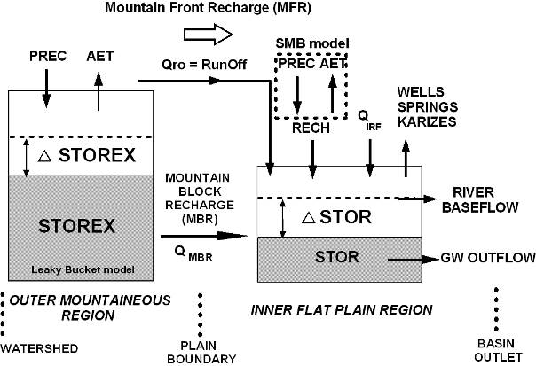
15Figure 1. Schematic presentation of the conceptual groundwater balance model.
16The watershed basin is divided into an inner, central, rather flat region (area 1), in which the aquifer system is developed (typically in the sedimentary filling of an old eroded valley) and a peripheral, mountainous outer region (area 2). A water balance is constructed for the inner region, with lateral inflow from the outer region, called mountain front recharge (MFR). The lateral inflow has two distinct contributions: a runoff component which reaches the inner region quite fast by (mountain) streams, and which feeds the aquifer in the central region by riverbed infiltration, and a second slower contribution by a subsurface groundwater cycle in the basement rock, called mountain block recharge (MBR). Net precipitation (PREC-AET) that falls in the outer region is fractioned into these two contributions using a single partitioning coefficient. Its value depends on topography in the outer region and hydraulic and hydrogeological properties of the bedrock. If the bedrock has a low hydraulic conductivity, most of the precipitation will be routed through runoff, but in karstified limestones (like in the Shahrekord case) the subsurface cycle can be more important. The amount of runoff inflow is calculated as the runoff fraction of net precipitation (PREC-AET). Lateral inflow by a groundwater cycle is slower. The inflow rate from this contribution is modelled using a leaky bucket model (Huang et al., 1996; Van den Dool et al., 2003). Groundwater storage in the outer area is traced by accumulating groundwater recharge into a buffer (STOREX). Outflow of the buffer is linearly proportional to the buffer size, and constitutes the MBR. With this mechanism MBR will also occur in dry periods (e.g. summer months) while storage in the outer region is slowly depleted as groundwater is discharged towards the central area. Depending on the rate factor MBRFCT, storage depletion in the mountain block region is faster (high outflow rates but fast decaying) or slower (more constant outflow rates). There is no upper limit on the buffer size, say storage capacity. The results of the application of the leaky bucket model to a recharge time series (from the Shahrekord region) is shown in figure 2. A value of 0.1/d for the rate coefficient is used in the example of figure 2 (but not in the calibrated model).
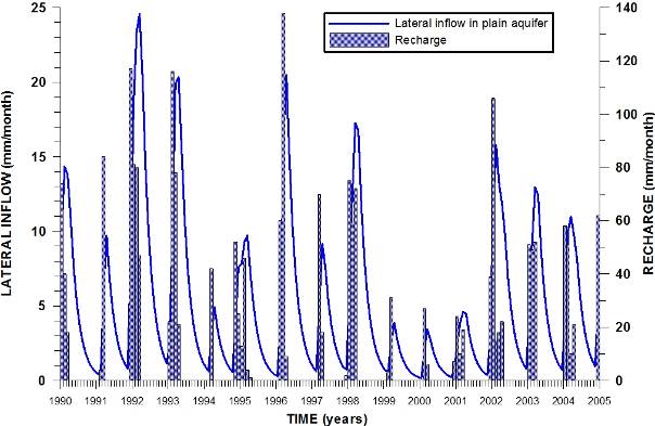
17Figure 2. Application of the leaky bucket model to the Shahrekord plain recharge: calculated lateral inflow and diffuse recharge.
18In the central region three main groundwater recharge balance components are distinguished. The first is diffuse recharge of the aquifer system originating from precipitation, the second is return flow from agricultural irrigation and a third component is the MFR from the outer region. Irrigation return flow is considered a fraction of total groundwater extraction and the fraction value was determined by model calibration.
19The main discharge component is groundwater exploitation like pumping and/or the use of water from wells. Water can leave the basin through river outflow or by subsurface flow. The lumped parameter model incorporates a mechanism through which river drainage is calculated when average piezometric level is above a predefined drainage level. Balancing the different components gives the change in groundwater storage in the central area. Changes in storage can be rescaled to changes in piezometric level by dividing by the areal extent of the inner region and the specific yield of the aquifer, which is obtained by model calibration.
20The water balance is conceived as a lumped parameter model which requires only a limited parameterisation. The used values should be representative for spatially averaged fields.
2.3. Groundwater balance equations
21The groundwater balance is only constructed for the aquifer system inside the basin plain, not for the whole watershed, and is obtained by integration of incoming and outgoing water fluxes over time. For a certain time period Δt this means:
22(Qin (m3/d) + Qout (m3/d)) x Δt (d) = ΔS (m3)
23Where: Qin are incoming water fluxes, Qout the outgoing fluxes (in m3/d) and ΔS is the change in water storage (in m3).
24The incoming fluxes are the sum of diffuse aquifer recharge (QRECH, inm3/d), irrigation return flow (QIRF, inm3/d) and lateral inflow from the surrounding mountains (subsurface and superficial, QMFR, inm3/d):
25Qin = QRECH + QIRF + QMFR
26Diffuse recharge from precipitation can be estimated from the soil moisture balance approach as proposed by Thornthwaite & Mather (1955, 1957). Potential evapotranspiration (PET) values can easily be estimated using the Thornthwaite equation which requires only temperature data, but these are lower than values obtained with other methods like Penman (Bakundukize et al., 2011) or Blaney-Criddle. Loukas et al. (2005) compared monthly PET values calculated with the equations of Thornthwaite, Blaney–Criddle (Allen et al., 1998), and the modified Penman–Monteith method (Penman, 1948; Monteith, 1965) for basins in Greece and found that the Thornthwaite values were systematically lower. The soil moisture balance method computes the actual evapotranspiration (AET) from the PET, depending on soil water availability.
27Irrigation return flow QIRF (inm3/d)is quantified as a fraction IRFCT of the total groundwater extraction QEX (inm3/d) inside the plain.
28QIRF = QEX*IRFCT
29Lateral inflow QMFR is thesum of the runoff from the mountains QRO (which infiltrates through the riverbeds) and subsurface flow QMBR (flow through the basement rocks, mountain block recharge):
30QMFR = QRO + QMBR = FF*(PREC-AET)*area2+(1-FF)*(ΔSTOREX+(PREC-AET))*area2*MBRFCT
31With:
32PREC = precipitation
33PET = potential evapotranspiration
34AET = actual evapotranspiration: if PREC > PET then AET = PET, if PREC < PET then AET = PREC+ΔSM, with SM = soil moisture)
35FF = fractioning factor between surface and groundwater flow (between 0 and 1)
36MBRFCT = hydraulic factor in leaky bucket model
37area2 = areal extent of peripheral, mountainous region between watershed boundary and plain boundary
38The outgoing component is the sum of groundwater extraction from the plain (QEX), water drained to the river network and subsurface groundwater outflow out of the basin (QSUB):
39QOUT = QEX+QRIV+QSUB
40Total groundwater exploitation QEX is the sum of groundwater taken by wells, springs and underground galleries (karizes, often used for capturing groundwater in semi-arid regions). River drainage is quantified by comparing average groundwater level LVL with an average drainage level in the streams (LVLDRN). If LVL > LVLDRN then the discharge to the river is calculated as the drain rate to bring the piezometric level at the river drainage level:
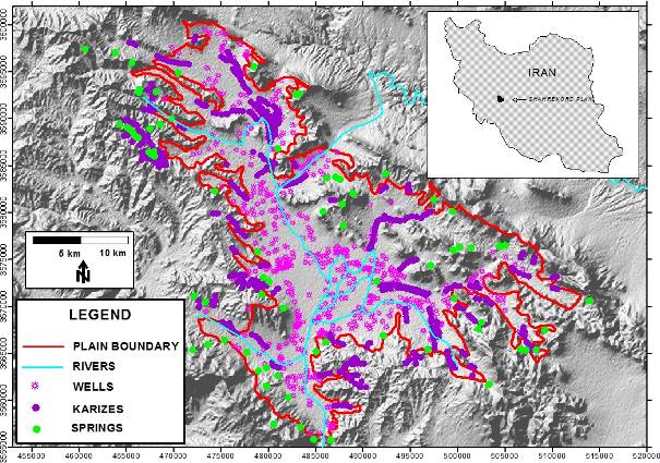
41QRIV=(LVL - LVLDRN)*area1*Sy
42With:
43LVL = average piezometric level at time t
44LVLDRN = defined average stream drainage level
45area1 = areal extent of the plain
46Sy = specific yield of the phreatic aquifer
47Average drainage levels can best be obtained by comparing calculated flow rates with measured river baseflow rates during the calibration period. Changes in piezometric levels in the model are proportional to changes in groundwater storage and are expressed with reference to predefined initial values at the start of the simulation.
48The average change in groundwater level (over the plain) is calculated by dividing the change in storage ΔS by the area of the plain (in m2) and by the specific yield of the phreatic aquifer Sy:
49Δlevel = (ΔS/area1) / Sy
50Assome of the groundwater balance components (Table 1) must be obtained from field data or groundwater statistics (exploitation amounts), they are only available as yearly totals. The model can be run with time steps of one year. However, using a soil water balance method for estimating groundwater recharge requires smaller timesteps such as months or even days if the appropriate data (such as precipitation) are available.
|
parameter |
type |
description |
|
QRECH |
Recharge |
Diffuse recharge in inner region by precipitation |
|
QMFR |
Recharge |
Lateral inflow from outer region |
|
QIRF |
Recharge |
Irrigation return flow |
|
QEX |
Discharge |
Groundwater exploitation (wells, springs, karizes) |
|
QRIV |
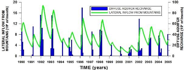
Discharge |
River outflow out of basin |
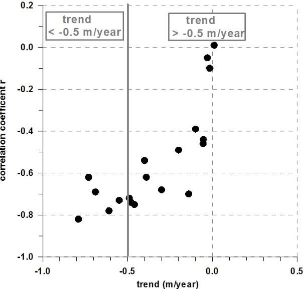
|
QSUB |
Discharge |
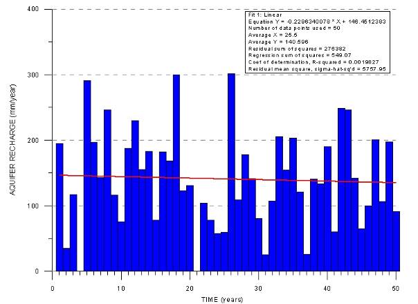
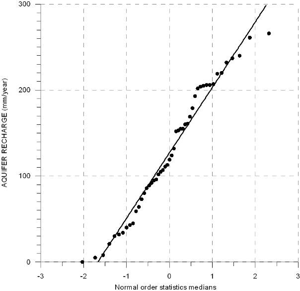
Subsurface flow over the basin outlet |
|
STOR |
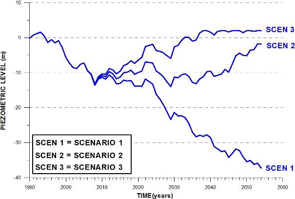
Storage |
Groundwater storage in inner region (area 1) |
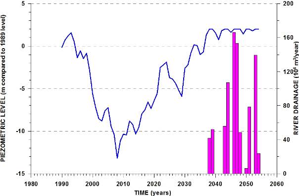
|
STOREX |
Storage |
Groundwater storage in outer region (area 2) |
51Table 1. Water balance parameters.
2.4. Soil moisture balance model
52Aquifer recharge (RECH) is estimated using a soil moisture balance, as described by Thornthwaite & Mather (1955). Soil moisture content in a soil ranges between a minimum SMmin (the permanent wilting point) and a maximum value SMmax (field capacity) and percolation of water can only occur when the soil is at field capacity. To calculate wetting and drying of the soil, an exponential relation between the soil moisture SM and the accumulated potential water loss (APWL) is assumed. APWL is the accumulated sum of previous PET-PREC values when PET was higher than precipitation PREC. Here, the implementation of the method by Willmott (1977) is used. Model input consists of precipitation and temperature data, model output includes PET and AET values and calculated aquifer recharge.
2.5. Model implementation
53The routines for the balance equations are implemented with the R programming language (Venables et al., 2009), but the calculations can easily be done in a spreadsheet. The model is conceived as a lumped parameter model, so no spatial variation of the input parameters is considered. The model requires in general nine input parameters (Table 2). The areal extent of inner and outer region depends on geography and topography. The parameters Sy, FF (fractioning factor between surface and groundwater flow in outer area), IRFCT (irrigation return flow fraction) and MBRFCT (hydraulic factor in the leaky bucket model) depend mainly on the hydrolithology and hydrostratigraphy of the aquifer system. Initial water levels and initial groundwater storage can be taken at zero at the start of the simulation. Changes in storage and piezometric level are then expressed compared to the initial state. The drainage level must be derived from observed baseflow and piezometric data. For each time step in the calculation of the model, precipitation, PET, aquifer recharge, groundwater extraction (in inner and outer region), must be entered.
|
Parameter |
Definition |
units |
|
Area1 |
Area of inner region (m2) |
m2 |
|
Area2 |
Area of outer region (m2) |
m2 |
|
Sy |
Specific yield of phreatic aquifer (-) |
- |
|
FF |
Fractioning factor between surface and groundwater flow in outer area |
- |
|
IRFCT |
Irrigation return fraction (-) |
- |
|
MBRFCT |
Constant in the leaky bucket model |
1/d |
|
LEVINI |
Initial average groundwater level (can be zero as reference) |
m |
|
STORINI |
Initial groundwater storage (can be zero as reference) |
m3 |
|
LVLDRN |
Level above which river drainage starts |
m |
54Table 2. General parameters required by the model.
2.6. Application to the Shahrekord basin
2.6.1. Description of the region
55The model has been applied to the Shahrekord basin in Iran (Radfar, 2009). Shahrekord plain is a 650 km2 sized sedimentary basin in central Iran (Fig. 3), located at a height between ca 2000 and 2300 masl, and surrounded by mountains and hills that can reach elevations in excess of 3000 masl. The topographic slope of the plain is from north to south. The plain is drained by a hydrographic network, and outflow out of the basin is through a narrow saddle at the south side of the basin. Flow rates in the main river at the outlet are strongly seasonal and limited to rainfall days in the wet season. Most of this is peakflow from surface runoff in the surrounding mountains. Baseflow is nearly non existent. However, in historic times river flow was more continuous.
56Figure 3. Topographic map of Shahrekord basin with location of wells, springs and karizes.
57The bedrock basement consists of limestone rocks that may locally be karstified. It is known that at some places karstic channels exist with intense flow. Sedimentary filling of the basin can reach a thickness of more than 100 m in the centre and consists of sandy and silty sediments. The upper part of the aquifer system is more silty. In the north of the basin a local aquitard occurs in the deeper parts of the aquifer system.
58According to the Köppen classification (Peel et al., 2007), the climate of the area is semi-arid, with a mean annual rainfall of 321 mm and a mean annual air temperature of 11.8 °C. Two different seasons can be distinguished. Most of the precipitation falls in winter months between November and April (Table 3). The coldest month is January with an average temperature below zero (-1.5 °C). About 40% of the precipitation occurs as snow. The dry season starts in June and has nearly no precipitation at all till October. Average temperature rises till 24 °C in July. Winter season has 50% of total precipitation, autumn 28% and spring 22% in Shahrekord station. Summer is nearly dry.
|
month |
Precipitation (mm) |
Average T (°C) |
Average H Humidity (%) |
|
Jan |
60.8 |
-1.5 |
67 |
|
Febr |
47.9 |
1.2 |
67 |
|
Mar |
60.3 |
6.0 |
62 |
|
Apr |
37.5 |
11.3 |
55 |
|
May |
14.1 |
15.9 |
48 |
|
Jun |
0.9 |
20.7 |
42 |
|
Jul |
1.9 |
24.0 |
33 |
|
Aug |
0.4 |
23.1 |
31 |
|
Sep |
0.0 |
18.8 |
32 |
|
Oct |
6.9 |
13.2 |
42 |
|
Nov |
32.2 |
7.4 |
54 |
|
Dec |
58.6 |
2.2 |
63 |
59Table 3. Long-term monthly averages of precipitation, temperature and humidity in Shahrekord station.
60Since 1984 a monitoring network of 19 observation wells is used to measure water levels biweekly. In the plain groundwater flow is from the north to the south, but the basin outlet is very narrow and groundwater outflow will be very limited. As the basin is surrounded by mountains only inflow through the bottom of the basin by mountain front recharge is considered. Therefore, hydrodynamically, the basin is rather closed and the water balance will be very sensitive to groundwater discharge inside the plain. Many piezometric time series show a steady decline in levels, more pronounced in the years 1999-2001. At some places levels have dropped around 10 m during the last decade. Figure 4 shows a representative time series of an observation well where the steady decline in levels in clearly visible. Superimposed is a seasonal cyclicity characterised by a rise in levels in wintertime by rainfall recharge and a decline in summer season because of intensive pumping for irrigation.
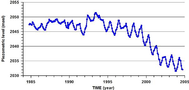
61Figure 4. Example of a piezometric time series (1984-2005).
62Agricultural development has lead to an increased demand in irrigation water. Since historic times, underground galleries (karizes) have been used to conduct water from the periphery of the plain into the central section. The location of these galleries can be derived from the position of shafts that are present. Also water from springs is used. Additionally wells have been dug. These were initially operated by hand, but their use has intensified after the introduction of mechanical pumps. Today more than 500 wells are operational in the plain. Most of these are located around cultivated land parcels. These form around 30.8% of the total area of Shahrekord plain. Statistics of the evolution of the number of wells are available. The number of installed wells may be indicative for the intensity of groundwater exploitation. Considering the large amounts of water that are used for irrigation, a significant fraction may re-infiltrate as irrigation return flow. Total groundwater exploitation is now equivalent to a discharge flux between 200 and 400 mm/year (Fig. 5). The location of the wells, karizes and springs is given on the map of figure 3.
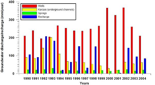
63Figure 5. Evolution of aquifer recharge and groundwater exploitation from wells, karizes (underground channels) and springs (1990-2004).
2.6.2. Application of the model
64The model has been run by using monthly time steps. To prepare the datasets on a monthly basis, some assumptions necessarily have been made. For each time step, the amounts for most of the water balance components have been defined, while other components have been quantified by model calibration (Table 4).
|
Balance component |
type |
Origin of data |
|
QRECH |
recharge |
Meteorological data and SMB |
|
QIRF |
recharge |
Model calibration, fraction of QEX |
|
QMFR |
recharge |
Model calibration |
|
QEX |
discharge |
Registered data |
|
QRIV |
discharge |
Absent in present situation |
|
QSUB |
discharge |
Neglected because very small |
65Table 4. Recharge and discharge water balance components in the model.
66Recharge components
67Recharge from precipitation was estimated with the soil moisture balance model WATBUG (Willmott, 1977) based on the Thornthwaite & Mather (1955) method, using precipitation and temperature data of Shahrekord city (Peterson & Vose, 1997) (available from 1956 to 2006). The water holding capacity was estimated at 100 mm by comparing the results of calculations with different values with the piezometric time series and the occurrence of recharge events. Results of the WATBUG model are presented in figure 6, showing:
68(i) measured monthly precipitation (bar chart) and calculated potential evapotranspiration (PET, thin solid line) and actual evapotranspiration (AET, thick solid line) values (top graph)
69(ii) calculated aquifer recharge (central graph)
70(iii) calculated soil moisture content (lower graph). The soil moisture at permanent wilting point is to be added to the values shown.
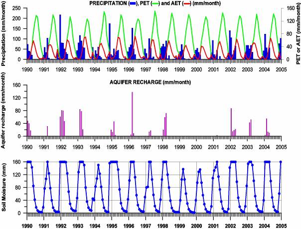
71Figure 6. Results of the WATBUG soil moisture water balance model (1990 - 2004).
72Over the period 1956-2006 average precipitation was 321 mm/year with an average calculated aquifer recharge of 123 mm/year.
73Irrigation return flow is considered a fraction of the total groundwater exploitation. The fractional value was obtained by model calibration and taken as a constant over time. Lateral inflow is estimated by using the leaky bucket model based on meteorological data and the size of the outer part of the basin (outside the plain). The factor relating storage with bucket outflow was found by model calibration.
74Discharge components
75The most important discharge component is groundwater extraction from wells, karizes and springs. Yearly totals are available from official statistics. In the monthly model, these exploitation rates were restricted to the dry season (April till September) and yearly totals were equally distributed over this six months’ period.
76As the river draining the basin is usually dry at the basin outlet, no large amounts of water leave this way. Only in winter months, after rainy periods, surface flow is observed and sporadic flow measurements are available since 1999. These are usually lower than 2 m3/sec and last no longer than a few days after rain events (Radfar, pers. comm.). Most of this water will be peakflow. Baseflow (QRIV) leaving the basin is considered negligible in the present situation. Subsurface groundwater outflow (QSUB) was estimated based on the hydraulic gradient observed at the south end of the basin and applying Darcy’s law. Amounts were small compared to the other balance components and were therefore not considered in the calculations. If necessary they can be prescribed in the model’s input file.
3. Results and discussion
3.1. Model calibration
77Model calibration was done using the NLM optimisation routine available in the stats package in R. Three parameters were determined: specific yield of the phreatic aquifer (Sy), irrigation return flow fraction (IRFCT) and the rate coefficient in the leaky bucket model for lateral inflow (MBRFCT). The parameter FF that controls the ratio of net precipitation that is diverted as runoff, was set to zero as (in this case) the model was quite insensitive for that parameter, as this water always enters into the aquifer system, by lateral inflow or as runoff that enters the plain and infiltrates locally. Calculated monthly piezometric levels were compared with the averages from the water level measurements in the 19 wells of the monitoring network. Minimizing the squared differences was the objective function. All observations had the same weighting factor.
78Calibrations were done with a subset of the observation series, using the first 8, 10 or 12 years of observation data. The remaining part of the series was then used to evaluate the model by comparing predicted values with the corresponding part of the observation data. An additional calibration was done using the whole series, but in this case no predictions can be done to control the models performance. The obtained parameter values are listed in Table 5. The specific yield Sy and MBRFCT parameter (controlling lateral inflow from the mountains) are becoming smaller as the length of the calibration series increases: specific yield is ca 14% while MBRFCT is around 0.12 day-1. The irrigation return fraction is in most calibrations nearly 10%.
|
#years used for calibration |
Sy |
IRFCT |
MBRFCT (1/d) |
|
8 |
0.179 |
0.100 |
0.177 |
|
10 |
0.131 |
0.077 |
0.195 |
|
12 |
0.144 |
0.103 |
0.137 |
|
15 |
0.141 |
0.105 |
0.119 |
79Table 5. Model parameter values obtained by model calibration using a subset of the observation series.
80The calculated piezometric series for the calibration runs are presented in figure 7. All calibration runs have too low levels in the first 3 to 4 years (1990-1994). The reason may be that aquifer recharge is underestimated in these years, related to the monthly time discretisation in the SMB method, while precipitation is concentrated in a limited number of high rainfall events on a few days. Between 1994 and 2000 the agreement is quite good. The declining trend in water levels after 2000 is reproduced by all calibrations, although levels in the last years are too high for the shorter calibrated models. Even the 8 years calibrated model, only based on data from before 2000, does predict the downward trend. The 15 years’ calibration has piezometric levels comparable with the 12 years’ fit. The deviation between calculated and measured values during the calibration period is listed in Table 6. For the 12 years’ fitted model, average deviation is around 40 cm.
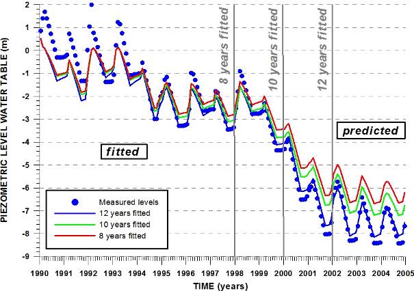
81Figure 7. Monthly observed and model simulated piezometric levels for calibrations with 8, 10 and 12 years of data.
|
#years used for calibration |
Length of calibration series (values) |
AAER (m) |
AER (m) |
|
8 |
96 |
0.507 |
-0.214 |
|
10 |
120 |
0.454 |
-0.236 |
|
12 |
144 |
0.428 |
-0.289 |
|
15 |
180 |
0.375 |
-0.229 |
82Table 6. Deviations between calculated and measured piezometric levels in the calibration interval (AAER = average absolute error, AER = average error).
83When the calibration period is shorter than 15 years, the remaining part was predicted with the model and deviations calculated with measurements (Table 7): average absolute errors (AAERR) and average errors (AERR). These errors are rather large for the 8 and 10 years’ calibrations, but decrease for the 12 years’ calibration. In that case the average error on 3 years ahead predictions (between years 12 and 15) is less than 20 cm. For this calibration the deviation is larger in the calibrated period than in the prediction interval (compare Tables 6 and 7). This is mainly due to the large deviations in the first years where computed levels are too high.
|
#years used for calibration |
Length of prediction series (values) |
AAER (m) |
AER (m) |
|
8 |
84 |
1.081 |
1.052 |
|
10 |
60 |
0.879 |
0.877 |
|
12 |
36 |
0.186 |
0.076 |
84Table 7. Deviations between calculated and measured piezometric levels in the prediction interval (AAER = average absolute error, AER = average error).
3.2. Model results
85The results for the 15 years’ calibrated model are considered. The monthly values for the main water balance components are accumulated into yearly totals (Fig. 8). Comparison of the main input components (aquifer recharge and lateral inflow from the mountains) and groundwater extraction (from wells, karizes and springs summed up) (Fig. 8) shows that in 7 of the 15 years the groundwater balance was negative, resulting in a decrease of the total storage. Initially, the wet winters of 92/93 and 93/94 resulted in a positive water balance, but the following years were dryer with a negative balance which lowered the average water level in the aquifer with around 2 meters. The positive balance of 1996 was insufficient to restore the 2 m drawdown, which was also not possible by 1997 which had a deficit in the balance. The wetter year 1998 could despite its positive balance only stabilize levels. Between 1994 and 1998 average groundwater level was around 2 m lower than in the period 1990-1994. The following 3 years showed a dramatic change in the piezometric evolution. The years 1999, 2000 and 2001 were three consecutive dry years with strong negative balances, mainly because of the very limited aquifer recharge. Yearly deficits ranged between 100 and 200.106 m3/year. This caused a global depletion of the aquifer storage with around 400.106 m3 and introduced a systematic lowering of the groundwater levels with 4 m. The years 2002, 2003 and 2004 had rather normal precipitation and recharge rates, but this could not rise water levels again, only stabilize the situation. To reverse the trend with the present exploitation going on further, a series of consecutive abnormally wet years would be necessary.
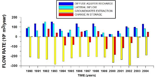
86Figure 8. Yearly accumulated water balance components for the 15 years’ calibrated monthly model run.
87The monthly values of diffuse aquifer recharge and lateral inflow from the surrounding mountains (MBR) are visualized in figure 9. Lateral inflow is a fluctuating function with peakflow at the end of the winter season. During winter period inflow increases fast and can double or triple in 2 or 3 months. Peak values depend strongly on the amount of rainfall and range between ca 4 and 18.106 m3/month. After the rainy season, the inflow drops according to an exponential decay function and reaches a minimum at the end of summer, usually between 2 and 4.106 m3/month. The highest inflow took place in the wet winters of 92/93 (ca 19.106 m3/month) and 93/94 (ca 17.106 m3/month). The lowest inflow occurred in 1999, 2000 and 2001 (ca 2.106 m3/month) when also winter peak values were very low. Average MBR inflow (1990-2004) is 6.67.106 m3/month, while the average plain diffuse aquifer recharge is 7.76.106 m3/month, but occurs only seasonally. Both are of comparable magnitude.
88Figure 9. Monthly values for lateral inflow from mountains and diffuse aquifer recharge in the 15 years’ calibrated monthly model run.
89Change in aquifer storage can act as a sink or a source term in the groundwater balance, as piezometric levels increase or decrease. Changes in storage are computed by the model, but can also be approximately derived from the evolution of piezometric levels in the time series of the 19 observation wells. Nearly all the observation wells show a declining trend and 5 out of the 19 wells have an average decreasing trend of more than half a meter a year (Fig. 10). Average trend is 0.34 m/year. Using this value as the representative trend for the whole plain with an area of 650 km2 and using a specific yield value of 12% (average of the values found from model calibration), yearly depletion of groundwater storage in the plain aquifer can be estimated at around 26.52.106 m3/year (= 650.106 x 0.34 x 0.12 m3/year). With a long term (1956-2006) average aquifer recharge of 128 mm a year (computed with the SMB model), total replenishment of the aquifer system by precipitation alone will be 83.2.106 m3/year. The yearly storage depletion is around one third of the normal aquifer replenishment in the plain.
90Figure 10. Linear trend and correlation coefficient in the 19 wells of the monitoring network.
3.3. Predictive scenario analysis
91In the period 1990-2004 average groundwater exploitation was 231.11.106 m3/year in the plain. Based on this number three predictive runs were done. First a continuation of the average exploitation rate is considered, and two gradual reduction schemes were applied: one with a yearly 1% and another with a yearly 2% reduction in exploitation (compared to the previous year). This means that in 50 years, exploitation will be reduced to 60% in the case of the second scenario and to less than 40% for the third scenario.
92Aquifer recharge in the predictive runs is not based on average meteorological conditions but derived from a generated rainfall series using a random sampler from a normal distribution with parameterisation derived from the measured rainfall yearly totals in Shahrekord city station. The series has no autocorrelation. With this series, aquifer recharge was calculated with the WATBUG model. The generated aquifer recharge time series has an average of 128.3 mm/year with a standard deviation of 74.7 mm (Fig. 11). The values are quasi normally distributed as can be seen on the QQ-plot (Fig. 12).
93Figure 11. Generated 50 years’ series of aquifer recharge used in the predictive scenario simulations.
94Figure 12. QQ-plot of yearly aquifer recharge (1956-2004).
95The predictive runs start in 2005, directly after the calibration period. However, since 2005 until present, no limitation on groundwater exploitation has been implemented. The results of these predictive runs are presented as the evolution of the average piezometric level over time (Fig. 13). Scenario 1 shows that with no restrictions on exploitation rates it can be expected that water levels will keep dropping with 25 m over the simulated 50 years. The second scenario with a yearly reduction of 1% will stabilize groundwater levels around the present situation. A very slow and partial recovery may be expected by the end of the considered period. According to scenario 3, a real recovery of the aquifer system would require a yearly reduction of 2% in exploitation rates (continuously over the next 50 years). Then, in around 35 years, levels will be restored and river drainage re-initiated. By then, baseflow at the basin outlet may become an important groundwater balance component (Fig. 14). Stream outflow during wet years may be as high as 100 to 120.106 m3/year.
96Figure 13. Calculated average groundwater levels in the predictive scenarios.
97Figure 14. Re-initiated river drainage in prediction scenario 3 and evolution of piezometric level compared to 1989.
4. Conclusion
98A lumped parameter groundwater balance model for aquifer systems located in intramountain basins has been developed and applied to an aquifer basin in Central Iran. The model is a lumped parameter model with a limited number of parameters, which is therefore easy to apply. In the model concept, lateral inflow from the surrounding mountains into the basin plain is an important balance component. Both surface runoff inflow and subsurface groundwater inflow are incorporated. The subsurface system is represented by a leaky bucket model. The lateral inflow, diffuse aquifer recharge (from rainfall) and irrigation return flow are considered as source components in the balance, while groundwater exploitation, outflow at the basin’s outlet and river drainage are sink terms. Changes in storage are derived from the groundwater balance and recalculated to changes in average piezometric level.
99The model was tested and run on data from the Shahrekord basin in Iran. This is an overexploited aquifer system where piezometric levels have dropped significantly during the last decade. Calibration runs using yearly and monthly data for the 15 years’ period 1990-2004 were performed to parameterise the model, using piezometric levels in 19 observation wells, distributed over the plain. The monthly based model can reproduce the seasonal cyclicity in the water budget and water levels.
100The calibrated model has been used to run three predictive scenarios. Continuation of the present exploitation rates will lower the piezometric levels with more than 25 m extra over the next 50 years. A decrease of exploitation rates with 1% each year over the next 50 years to around 60% of the present exploitation rate (around 2055), will stabilize the downward trend, with a slow partial recovery between 2040 and 2050. A decrease with 2% each year over the next 50 years to around 35% of the present value, will result in a gradual increase in water levels. Around 2040, original water levels will be restored and drainage by the river system re-initiated.
5. Acknowledgments
101The authors are grateful to the Ministry of Power of Iran, particularly offices in Charmahal and Bakhtiari Province, for providing support with data sets and field experiments, and to the Iranian Ministry of Science, Research and Technology and Shahrekord University for their financial support to Mahdi Radfar for doing his PhD research at Ghent University. We want to thank Dr. Maurizio Polemio and an anonymous reviewer for their comments, which helped us to improve the manuscript.
6. References
102Ajami, H., Troch, P. A., Maddock III, T., Meixner, T. & Eastoe, C., 2011. Quantifying mountain block recharge by means of catchment-scale storage-discharge relationships. Water Resources Research, 47(4), W04504.
103Allen, R.G., Pereira, L.S., Raes, D. & Smith, M., 1998. Crop evapotranspiration-guidelines for computing crop water requirements. Rome, Italy: Food and Agriculture Organization of the United Nations, FAO Irrigation and Dainage Paper 56.
104Bakundukize, C., Van Camp, M. & Walraevens, K., 2011. Estimation of groundwater recharge in Bugesera region (Burundi) using soil moisture budget approach. Geologica Belgica, 14(1-2), 85-102.
105Edmunds, M., Fellman, E., Goni, I. & Prudhomme C., 2002. Spatial and temporal distribution of groundwater recharge in northern Nigeria. Hydrogeology Journal, 10(1), 205-215.
106Eilers, V.H.M., Carter, R.C. & Rushton, K.R., 2007. A single layer soil water balance model for estimating deep drainage (potential recharge): An application to cropped land in semi-arid North-east Nigeria. Geoderma, 140, 119–131.
107Gebreyohannes, T., De Smedt, F., Walraevens, K., Gebresilassie, S., Hussien, A., Hagos, M., Amare, K., Deckers, J. & Gebrehiwot, K., 2013. Application of a spatially distributed water balance model for assessing surface water and groundwater resources in the Geba basin, Tigray, Ethiopia. Journal of Hydrology, 499, 110-123.
108Hibbs, B.J. & Darling, B.K., 2005. Revisiting a Classification Scheme for U.S.-Mexico Alluvial Basin-Fill Aquifers. Ground Water, 43(5), 750-763.
109Huang, J., Van den Dool, H.M. & Georgakakos, K.P., 1996. Analysis of model-calculated soil moisture over the United States (1931–1993) and applications to long-range temperature forecasts. Journal of Climate, 9, 1350–1362.
110Kao, Y., Liu, C., Wang, B. & Lee, C., 2012. Estimating mountain block recharge to downstream alluvial aquifers from standard methods. Journal of Hydrology, 426–427, 93–102.
111Kattan, Z., 2008. Estimation of evaporation and irrigation return flow in arid zones using stable isotope ratios and chloride mass-balance analysis: Case of the Euphrates River, Syria. Journal of Arid Environments, 72, 730–747.
112Keith, S.J., 1980. Mountain front recharge. In Wilson, L.G. et al. (eds), Regional recharge research for Southwest alluvial basins. Tucson, University of Arizona, pp. 4-1 to 4-44.
113Loukas, A., Vasiliades, L., Domenikiotis, C. & Dalezios, N.R., 2005. Basin-wide actual evapotranspiration estimation using NOAA/AVHRR satellite data. Physics and Chemistry of the Earth, 30, 69–79.
114Magruder, I.A., Woessner, W.M. & Running, S.W., 2009. Ecohydrologic Process Modeling of Mountain Block Groundwater Recharge. Ground Water, 47(6), 774-785.
115Manning, A.H., 2002. Using noble gas tracer to investigate mountain block recharge to an intermountain basin, PhD Thesis, University of Utah, Salt Lake City.
116Manning, A.H. & Solomon, D.K., 2003. Using noble gases to investigate mountain-front recharge. Journal of Hydrology, 275, 194–207.
117Manning, A.H. & Solomon, D.K., 2004. Constraining mountain-block recharge to the eastern Salt Lake Valley, Utah with dissolved noble gas and tritium data. In Hogan J.F., Phillips F.M. & Scanlon B.R. Groundwater recharge in a desert environment: The Southwestern United States. Water Science and Application 9, American Geophysical Union, Washington D.C., 139-158.
118Mjemah, I.C., Van Camp, M., Martens, K. & Walraevens, K., 2011. Groundwater exploitation and recharge rate estimation of Quaternary sand aquifer in Dar-es-Salaam area, Tanzania. Environmental Earth Science, 63, 559–569.
119Monteith, J.L., 1965. Evaporation and environment. Symposia of the Society for Experimental Biology 19, 205-224.
120Neilson-Welch, L., Allard, R., Geller, D., Hamilton, H., Uunila, L., Fioley, J. & Allen, D., 2009. A water balance approach for quantifying mountain front recharge (MFR). The Geological Society of America. Cordilleran Section Meeting - 105th Annual Meeting (7-9 May 2009). Kelowna, British Columbia.
121Peel, M.C., Finlayson, B.L. & McMahon, T.A., 2007. Updated world map of the Köppen–Geiger climate classification. Hydrology and Earth System Sciences, 11, 1633–1644.
122Penman, H.L., 1948. Natural evaporation from open water, bare soil and grass. Proceedings of the Royal Society of London A, 193(1032), 120-145.
123Peterson, T.C. & Vose, R.S., 1997. An overview of the Global Historical Climatology Network temperature database. Bulletin American Meteorological Society, 78, 2837– 2849.
124Portoghese, I., Uricchio, V. & Vurro, M., 2005. A GIS tool for hydrogeological water balance evaluation on a regional scale in semi-arid environments. Computers & Geosciences, 31, 15–27.
125Radfar, M., 2009. Hydrogeological and Hydrochemical Characterisation and Modelling of the Tertiary-Quaternary Aquifer System in Shahrekord Plain – Iran. PhD dissertation. Ghent University.
126Radfar, M., Van Camp, M. & Walraevens, K., 2013. Drought impacts on long-term hydrodynamic behavior of groundwater in the tertiary–quaternary aquifer system of Shahrekord Plain, Iran. Environmental Earth Sciences. 70(2), 927-942.
127Scanlon, B.R., Keese, K.E., Flint, A.L., Flint, L.E., Gaye, C.B., Edmunds, W.M. & Simmers, I., 2006. Global synthesis of groundwater recharge in semiarid and arid regions. Hydrological Processes, 20, 3335–3370.
128Stone, D.B., Moomaw, C.L. & Davis, A., 2001. Estimating recharge distribution by incorporating runoff from mountainous areas in an alluvial basin in the Great Basin region of the southwestern United States. Ground Water, 39(6), 807-818.
129Thiros, A., 1995. Chemical composition of ground water, hydrologic properties of basin-fill material, and ground water movement in Salt Lake Valley, UT. Utah Department of Natural Resources Technical Publication No. 110.
130Thornthwaite, C.W. & Mather, J.R., 1955. The water balance. Publications in Climatology 8(1), 1-104.
131Thornthwaite, C.W. & Mather, J.R., 1957. Instructions and tables for the computing potential evapotranspiration and the water balance. Publications in Climatology 10(3), 185-311.
132Van Camp, M., Coetsiers, M., Martens, K. & Walraevens, K., 2010a. Effects of multi-annual climate variability on the hydrodynamic evolution (1833 to present) in a shallow aquifer system in northern Belgium. Hydrological Sciences Journal.55(5), 763-779.
133Van Camp, M., Radfar, R. & Walraevens, K., 2010b. Assessment of groundwater storage depletion by overexploitation using simple indicators in an irrigated losed aquifer basin in Iran. Agricultural Water Management, 97, 1876–1886.
134Van Camp, M., Radfar, M., Martens, K. & Walraevens, K., 2012. Analysis of the groundwater resource decline in an intramountain aquifer system in Central Iran. Geologica Belgica 15(3), 176-180.
135Van Camp, M., Mjemah, I.C., Al Farrah, N. & Walraevens, K., 2013. Modeling approaches and strategies for data-scarce aquifers: example of the Dar es Salaam aquifer in Tanzania. Hydrogeology Journal, 21, 341-356.
136Vandecasteele, I., Nyssen, J., Clymans, W., Moeyersons, J., Martens, K., Van Camp, M., Gebreyohannes, T., Desmedt, F., Deckers, J. & Walraevens, K., 2011. Hydrogeology and groundwater flow in a basalt-capped Mesozoic sedimentary series of the Ethiopian highlands. Hydrogeology Journal, 19, 641–650.
137Van den Dool, H., Huang, J. & Fan, Y., 2003. Performance and analysis of the constructed analogue method applied to U.S. soil moisture over 1981-2001. Journal Geophysical Research, 108(D16), 8617.
138Venables, W.N., Smith, D.M. and the R development core team, 2009. An introduction to R. 2nd ed. Network Theory, 137 p.
139Walraevens, K., Vandecasteele, I., Martens, K., Nyssen, J., Moeyersons, J., Tesfamichael, G., De Smedt, F., Poesen, J. & Van Camp, M., 2009. Groundwater recharge and flow in a small mountain catchment in northern Ethiopia. Hydrological Sciences Journal, 54(4), 739-753.
140Welsh, W.D., 2007. Groundwater balance modelling with Darcy’s law. PhD thesis. A thesis submitted for the degree of Doctor of Philosophy of The Australian National University.
141Widén-Nilsson, E., Halldin, S. & Xu C., 2007. Global water-balance modelling with WASMOD-M: Parameter estimation and regionalisation. Journal of Hydrology, 340, 105– 118.
142Willmott, C.J., 1977. WATBUG: A FORTRAN IV algorithm for calculating the climatic water budget. Publications in Climatology, 30(2), 1-54.
143Wilson, J.L. & Guan, H., 2004. Mountain block hydrology and mountain front recharge. In Hogan, J.F., Phillips, F.M. & Scanlon, B.R. (eds), Groundwater Recharge in a Desert Environment: The Southwestern United States, Water Science and Applications Series, 9, 113–137. American Geophysical Union, Washington, DC.
144Wilson, J.L., Guan, H. & Goodwin, L.B., 2002. Modeling investigation of mountain front recharge from typical mountain blocks. GSA Annual Meeting Denver (October 27-30, 2002).
145Manuscript received 24.06.2014, accepted in revised form 05.05.2015, available on line 23.06.2015.
