


- Portada
- Volume 22 (2019)
- number 3-4
- Vertical and lateral distribution of Foraminifera and Ostracoda in the East Frisian Wadden Sea – developing a transfer function for relative sea-level change


Vista(s): 3886 (61 ULiège)
Descargar(s): 622 (9 ULiège)

Vertical and lateral distribution of Foraminifera and Ostracoda in the East Frisian Wadden Sea – developing a transfer function for relative sea-level change

Abstract
In light of rising sea levels and increased storm surge hazards, detailed information on relative sea-level (RSL) histories and local controlling mechanisms is required to support future projections and to better prepare for future coastal-protection challenges. This study contributes to deciphering Holocene RSL changes at the German North Sea coast in high resolution by developing a transfer function for RSL change. Recent associations of Foraminifera and Ostracoda from low intertidal to supratidal settings of the barrier island of Spiekeroog in combination with environmental parameters (granulometry, C/N, total organic carbon, salinity) were investigated and quantified in elevation steps of 15 cm in order to generate a first transfer function (TF) of Holocene RSL change. In a future step, the TF can be applied to the stratigraphic record. Our data show a clear vertical zonation of foraminifer and ostracod taxa between the middle salt marsh and the tidal flat with very few individuals in the sand flat area, suggesting removal by the tidal current or poor preservation. Multivariate statistics identify the elevation, corresponding to the inundation frequency, as main driving factor. The smallest vertical error (49 cm) is associated with an entirely new approach of combining Foraminifera and Ostracoda for a TF. Advantages of the TF over classical RSL indicators such as basal and intercalated peats – beside the relatively narrow indicative meaning – include the possible application to a wide range of intertidal facies and that the resulting RSL curve does not depend on compaction-prone peats.
Tabla de contenidos
1. Introduction
1Relative sea-level (RSL) reconstructions are essential for understanding past and recent coastal processes and represent a crucial framework for future predictions of sea-level rise (Woodroffe & Murray-Wallace, 2012). This information is urgently needed for all fields of coastal zone management and the mitigation of coastal hazards – in particular in light of rising sea levels and a future increase of storm surge levels (Weisse et al., 2012; Rahmstorf, 2017) –, as well as in the fields of basic coastal research (e.g. geomorphology, sedimentology, palaeoclimatology, geoarchaeology) (Overpeck et al., 2006; Nicholls & Cazenave, 2010). The reconstruction of Holocene RSL changes along the German North Sea coast, until now, is mostly based on basal and intercalated peats (e.g. Behre & Streif, 1980; Behre, 2007) and shows rather coarse vertical resolution. Several authors have expressed the need for more precise quantitative data (Vink et al., 2007; Bungenstock & Schäfer, 2009; Bungenstock & Weerts, 2010, 2012; Baeteman et al., 2011; Meijles et al., 2018).
2A high-resolution reconstruction of past local RSL changes can be achieved by means of analysis of fossil salt-marsh Foraminifera, shell-bearing protists, which create very specific assemblages in the sedimentary record based on habitat conditions. A dense dataset of taxa distribution along a vertical transect of local modern intertidal environments can be used to develop a transfer function (TF), which models the relation between elevations of sample points and relative abundances of foraminifer species over time. Such a TF may permit inferences of palaeo-water depths with a centimetre-scale precision (Leorri et al., 2010; Kemp et al., 2012; Edwards & Wright, 2015), but typically within ~10–15% of the tidal range, leading to a decimetre-scale precision for mesotidal environments (Barlow et al., 2013). The use of salt-marsh Foraminifera for local RSL reconstructions has been established during the last two decades especially in North America, Denmark and on the British Isles (e.g. Scott et al., 2001; Gehrels & Newman, 2004; Gehrels et al., 2002; Pedersen et al., 2009; Engelhart & Horton, 2012; Kemp et al., 2013), but so far, applications are lacking for the southern part of the German Bight. Besides Foraminifera, Ostracoda, small crustaceans with a bivalved calcified carapace, occur within the same sediment fractions in the wider study area (Scheder et al., 2018). We assume that Ostracoda may provide additional information for more detailed reconstructions for the lower intertidal and uppermost subtidal. For the first time in palaeo-sea-level research, we combine Foraminifera and Ostracoda for a RSL TF (relative sea-level transfer function).
3This study presents the vertical zonation of recent living and dead Foraminifera and Ostracoda along a cross-shore profile in the back-barrier tidal flat of the East Frisian barrier island of Spiekeroog as an initial step of a transfer function-based RSL reconstruction. Foraminifera and Ostracoda distribution is interpreted in light of tidal influence and sedimentary environments and translated into a first RSL TF. Research hypotheses are:
4A vertical and lateral zonation of associations of foraminifers and ostracods mainly depends on elevation, hence, the duration of water cover.
5The additional use of ostracods for TF development leads to an improvement compared to the common procedure of using exclusively foraminifers.
6A foraminifer and ostracod based TF provides a more precise vertical resolution of sea-level index points than so far used at the German North Sea coast.
2. Study area
7The study area is situated at the southern coast of Spiekeroog (Fig. 1), one of the East Frisian barrier islands, which developed after around 6–7 ka BP (kiloyears before present, i.e. before AD 1950) when the post-glacial sea-level rise decelerated (Behre, 1987; Freund & Streif, 1999; Flemming, 2002; Bungenstock & Schäfer, 2009). Due to ongoing RSL rise and prevalent longshore current directions, the barrier islands have shifted over several kilometres in a south-easterly direction since their formation (Streif, 1990; Flemming, 2002), reaching their recent position about 2000 years ago (Freund & Streif, 2000). Diurnal tides (mean tidal range = 2.7 m; BSH 2018) fill and empty the back-barrier mesotidal prism of Spiekeroog through the two tidal inlets Otzumer Balje and Harle. The tidal flat merges towards the island and transforms into a well-developed salt marsh. The area is characterised by a humid tempered climate (Cfb after latest Köppen-Geiger classification; Kottek et al., 2006; Beck et al., 2018) with mean winter temperatures between 2.9 and 5.7 °C and mean summer temperatures between 15.8 and 18.3 °C (weather station Wangerland-Hooksiel, survey duration: 2014–2019). The salinity lies around 30 psu (practical salinity units) close to the main tidal channel (southeast of the island) and a little lower towards the mainland. After occasional freshwater input (e.g. heavy rainfall events), the salinity can decrease to less than 25 psu (Kaiser & Niemeyer, 1999; Reuter et al., 2009).
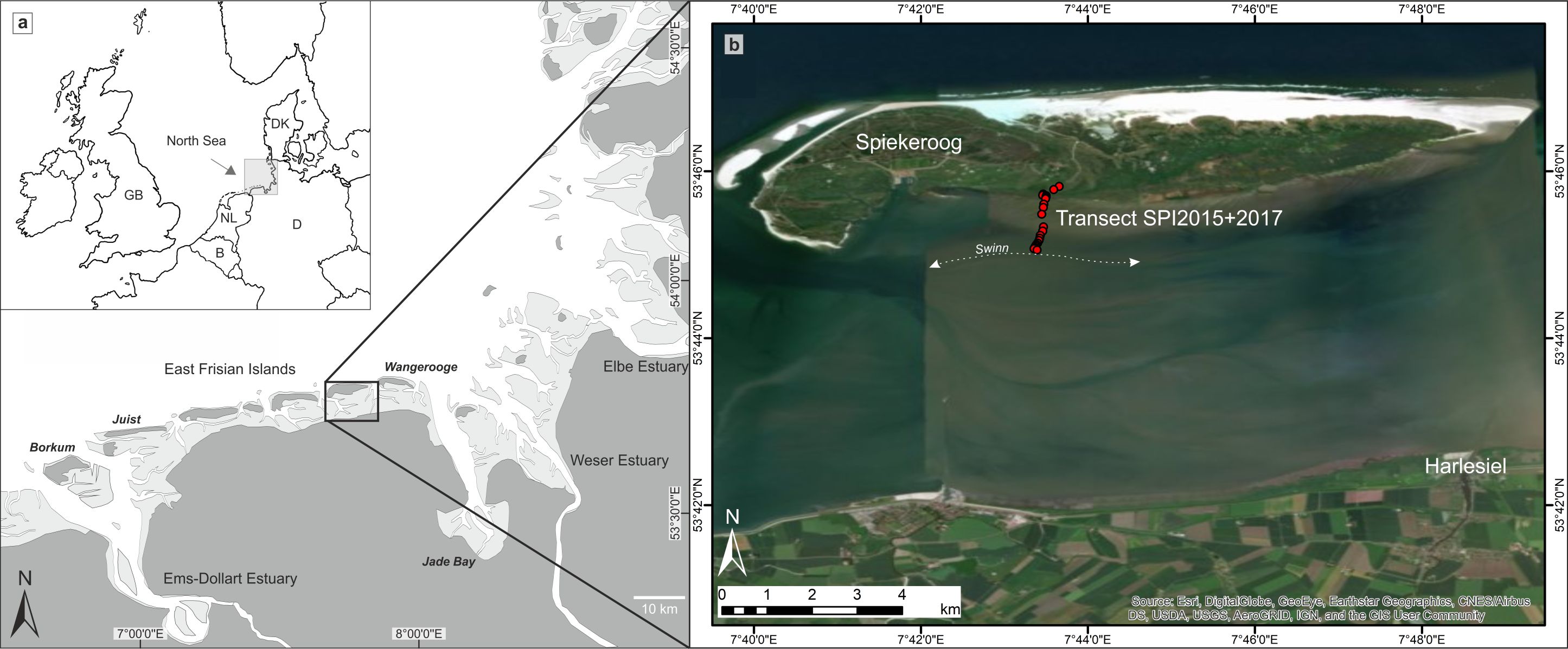
Figure 1. Overview of the study area. a: The southern North Sea coast with the East Frisian Islands (Spiekeroog is framed). b: The back-barrier area of Spiekeroog with the investigated surface transect at the southern coast of the island reaching from the salt marsh to the nearest tidal channel ‘Swinn’ (map source: Esri, Digital Globe, GeoEye, Earthstar Geographics, CNES/Airbus DS, USDA, USGS, Aerogrid, IGN, and the GIS User Community).
8Due to the shore-normal energy gradient (cf. Nyandwi & Flemming, 1995), an offshore-coarsening trend in grain sizes is observed. This general trend can be locally interrupted by tidal channels, depressions or old channel fillings (Bungenstock et al., 2002), whereas the barrier islands do not disturb it. Thus, there is no shoreward fining trend in grain size in the southern salt marshes of the island. Therefore, sampling in the opposite direction from the island’s salt marshes down to the low water line in the back-barrier tidal flat generally results in sampling from sand flats to finer-grained mixed flats. The investigated transect (c. 1180 m in N-S direction, directly bordering the national park area) covers the natural salt marsh and adjacent back-barrier tidal flat of the island reaching the nearest tidal channel ‘Swinn’ in the south (Figs 1 and 2). The vegetation above and along the transect shows a more or less characteristic pattern from the high to middle salt marsh (sea lavender [Limonium vulgare]) crossing the ‘Andel’ Zone (lower salt marsh; andel grass [Puccinellia maritima], salt bush [Atriplex halimus]) and the Glasswort Zone (pioneer zone; cord grass [Spartina anglica], glasswort [Salicornia europaea]) down to the Seagrass Zone (tidal flat; seagrass [Zostera]) (e.g. Streif, 1990; Gerlach, 1999).
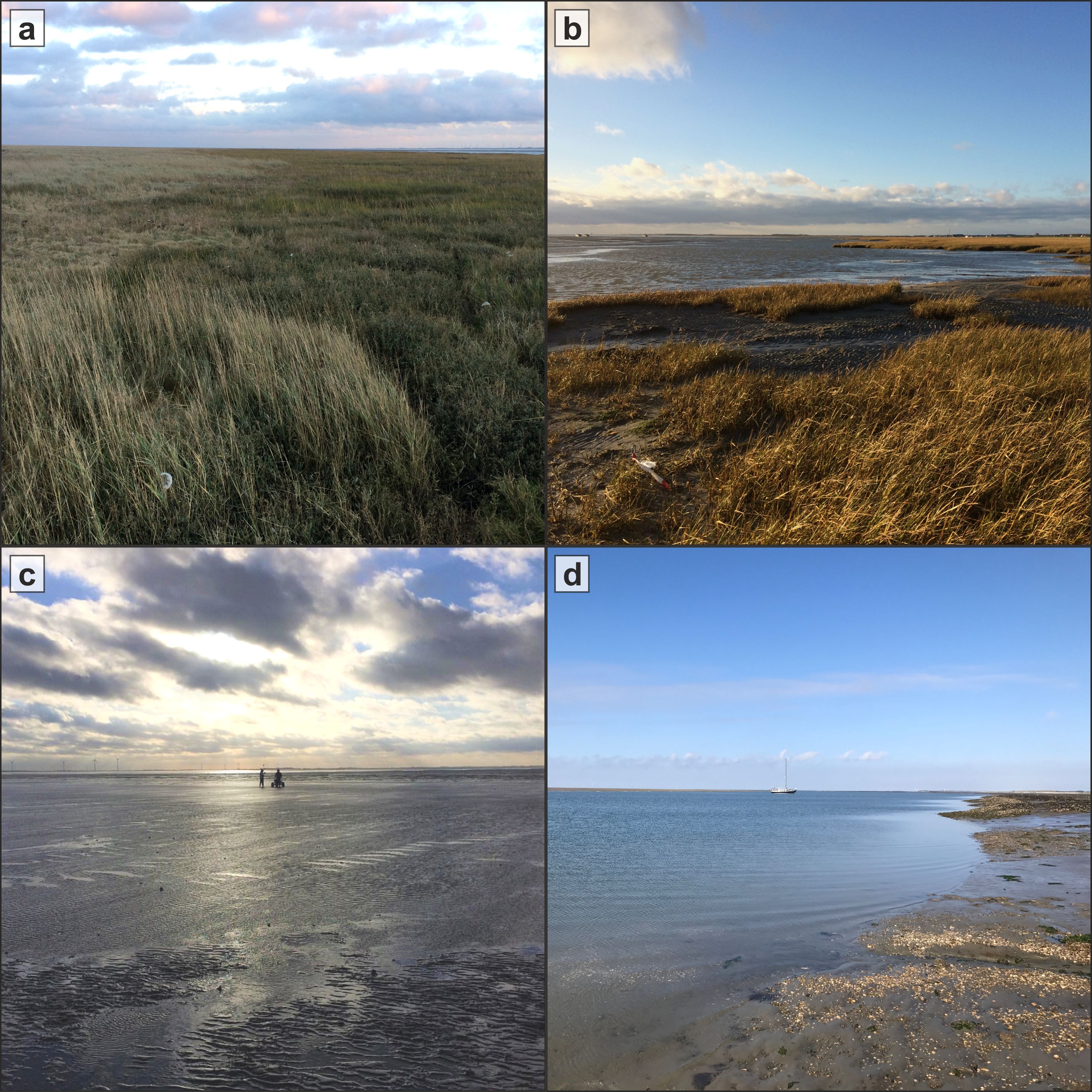
Figure 2. Photographic documentation of the study area during low tide. a: transition between middle and lower salt marsh (view towards SE); b: transition between salt marsh (pioneer zone) and sand flat (view towards W); c: view from the sand flat to the mixed flat (view towards S); d: margin of the tidal channel ‘Swinn’ (view towards SW).
3. Methods
3.1. Field work
9Twenty-three samples were taken during low tide (nineteen in December 2015 [neap-tide situation, 9–10 °C, dry weather], additional four in July 2017 [spring-tide situation, 15–20 °C, c. 1 mm of rainfall before sampling]) along a transect reaching from shallow subtidal (tidal channel levee) to supratidal (salt marsh) areas (Fig. 2) at the southern coast of Spiekeroog. Samples were taken in steps of 15 cm elevation difference with steel sampling rings (Eijkelkamp; diameter: 5 cm) comprising the uppermost 5 cm of the sediment surface. In order to distinguish living from dead individuals, samples were conserved with rose Bengal-coloured Ethanol (Walton, 1952; Edwards & Wright, 2015). At each sampling point, additional surface samples were taken for sedimentological analyses and, water coverage provided, water samples were taken in centrifuge tubes for salinity measurements in the laboratory. Elevation measurements at each sampling point were conducted using a differential global navigation satellite system (DGNSS; Topcon Hiper Pro). By anchoring the measured grid to the trigonometric point 2212 052 00 of the ‘Landesamt für Geoinformation und Landesvermessung Niedersachsen’ (LGLN) in the Spiekeroog salt marsh, the setup provides a vertical and lateral accuracy of ±2 cm. Since the 2017 transect is slightly shifted in N-S direction, samples had to be projected onto the 2015 surface profile (Fig. 3).
3.2. Laboratory analyses
10All microfaunal samples were carefully shaken overnight with a dispersant (sodium pyrophosphate; Na4P2O7 ; 46 g/l) to prevent adhesion of clay particles and afterwards washed through sieves, separating them into >63 µm and >100 µm fractions. For three representative samples the latter was split into eight aliquots per sample using a wet splitter after Scott & Hermelin (1993). From these aliquots a maximum of 200–300 individuals were counted wet in order to avoid drying of organic components and damaging of agglutinated Foraminifera (e.g. de Rijk, 1995; Edwards & Wright, 2015; Milker et al., 2016; Müller-Navarra et al., 2016). No species sensitive to drying were found in these samples and no damaging of tests could be observed after drying extracted individuals. Therefore, the remaining samples were air-dried, split with a micro splitter (ripple divider) and counted dry. The proportion of dry-counted material was weighed in order to enable extrapolation of microfaunal concentration per sample. Foraminiferal species were identified based on taxonomic descriptions and illustrations in Gehrels & Newman (2004), Horton & Edwards (2006) and Murray (2006), whereas identification of ostracod species followed the descriptions in Athersuch et al. (1989) and Frenzel et al. (2010). Because of the problem of discriminating juvenile individuals of Leptocythere, those species were grouped under Leptocythere spp. for counting. Discrimination of living and dead individuals was based on staining for foraminifers (at least one chamber stained = living; not stained = dead) and on well preserved soft parts in ostracods. The replacement of the genus Jadammina by Entzia is based on Filipescu & Kaminski (2011), who regard Entzia as a senior synonym of Jadammina. Foraminifer and ostracod associations were combined into a basic population for statistical analysis (100% = foraminifers + ostracods). After testing the detailed vertical distribution of living individuals for three representative samples, showing significant numbers of living individuals within the upper 3 cm, these were combined for microfaunal investigation and the lower 2 cm were discarded.
11Samples for sedimentological and geochemical analyses were dried at 40 °C and carefully pestled by hand. For grain-size analysis, carbonates were dissolved with hydrochloric acid (HCl; 10%) and organic matter removed using hydrogen peroxide (H2O2; 15%). In order to prevent aggregation, samples were treated with sodium pyrophosphate (Na4P2O7; 46 g/l). The grain-size distribution was determined on the <2 mm fraction using a laser particle size analyser (Beckman Coulter LS 13320) with a laser beam (780 nm) applying the Fraunhofer optical mode (Eshel et al., 2004). Since different species of Foraminifera and Ostracoda often prefer different substrates (cf. Frenzel et al., 2010), the microfaunal associations can be related to grain-size distribution.
12The organic content was determined by measuring the concentration of total organic carbon (TOC, constituting c. 50% of the organic matter). This was accomplished using an elemental analyser (elementar, Vario EL Cube), which enabled simultaneous measurements of nitrogen (N) and the determination of total inorganic carbon (TIC). The derived C/N ratio can provide information about the aquatic or terrestrial origin of organic matter (e.g. Last & Smol, 2001).
13The salinity was measured under laboratory conditions using a conductivity meter CO310 (VWR). Since the measurement was conducted with a delay of several months, the results are expected to be influenced by evaporation within the closed vessels. However, this should be consistent between all samples, so a general trend can be inferred.
3.3. Data processing
14The calculation of univariate statistical grain-size measures after Folk & Ward (1957) was carried out using GRADISTAT software (Blott & Pye, 2001). As preparation of the data set for multivariate analyses, Pearson correlation coefficients were calculated between the environmental parameters (sand amount, mean grain size, TOC, TIC, N, C/N, elevation) and microfaunal data in order to detect possible auto-correlations. The distributions of foraminifer and ostracod taxa as well as standardised environmental parameters were analysed by means of multivariate statistics (PCA, CCA, DCA) in order to evaluate driving environmental parameters and test whether species show unimodal or linear response along the main environmental gradient. Both correlation and multivariate statistics were performed using the software PAST (v. 3.21; Hammer et al., 2001). Afterwards, the TF was developed from the training data using the software C2 (v. 1.7.7; Juggins, 2007). According to the gradient length revealed by the DCA (3.3 standard deviation [SD]), a more unimodal species-environment relation can be expected (Birks, 1995; Lepš & Šmilauer, 2003), wherefore modelling was conducted using the weighted averaging-partial least squares (WA-PLS) method. To avoid overfitting, a maximum of three components was modelled (cf. Kemp & Telford, 2015). Bootstrapping cross-validation (1000 cycles) was used to evaluate the TF performance based on the coefficient of determination (R²boot), providing an estimation of the grade of the linear relationship between observed and estimated elevations in the training set, and the root mean squared error of prediction (RMSEP), enabling the evaluation of the general predictive capability of the TF (Milker et al., 2017). The most appropriate of the three modelled components was chosen based on the lowest RMSEP and highest R²Boot. Visual presentation of the data was accomplished by means of the software Grapher (v. 8.0.278) and the drawing application CorelDRAW X8 (v.18.1.0.690).
4. Results of microfaunal, sedimentological and geochemical investigations
15The investigated transect reaches from 53°45’42.27’’ N, 7°43’27.76’’ E (1.51 m NHN [m above Normalhöhennull = standard elevation zero referring to gauge Amsterdam]) in the north to 53°45’2.32’’ N, 7°43’23.49’’ E (-1.31 m NHN) in the south (Fig. 3). The separation of six zones (Zones A–F) was carried out based on qualitative interpretation of sedimentary (in particular grain-size distribution, TOC) and microfaunal (in particular foraminiferal abundance and composition) data in combination with field observations (Figs 3 and 4). Zone boundaries were defined in between two samples by considering the mean elevation between them. Foraminifer and ostracod species are always mentioned in ranking order concerning their abundances. In total, eight foraminifer and three ostracod taxa (Plate 1) were identified in both living and dead fauna. In general, much less living than dead individuals occur and microfaunal densities vary strongly between zero and 2500 ind./10 cm³ (individuals per 10 cm³) throughout the transect.
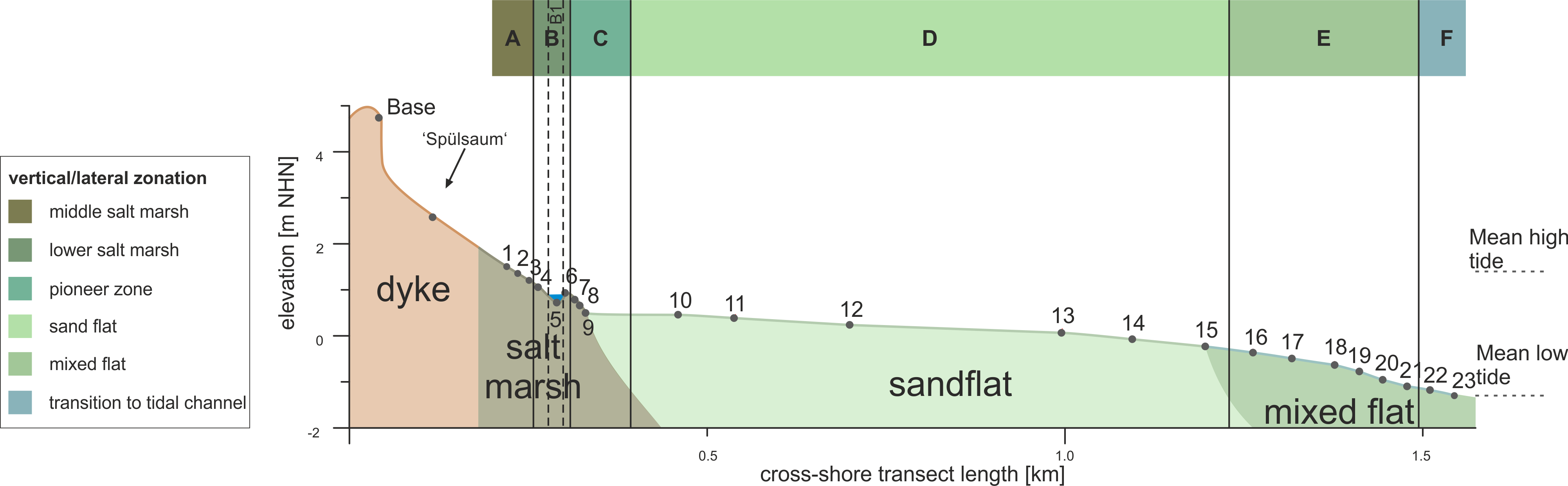
Figure 3. Elevation profile of the investigated surface transect showing sampling points, landscape units observed in the field as well as the identified zonation.
16Zone A (middle salt marsh), comprising the northernmost three samples (c. 1.51–1.13 m NHN; samples 1, 2 and 3) is characterised by very poorly sorted sandy mud in the upper and muddy sand in the lower part. The vegetation is characterised by Limonium vulgare (sea lavender) and Puccinellia maritima (andel grass). TOC and TIC values show opposite trends with TOC decreasing and TIC increasing towards lower elevations. The N content and the C/N ratio both decrease towards lower elevations. No water cover was present. The microfaunal composition is characterised by high diversity and high abundance (up to c. 2200 individuals/10 cm³). Foraminifers are dominated by Triloculina oblonga (Montagu, 1803) in the upper and Ammonia tepida (Cushman, 1926) in the lower part, followed by Haynesina germanica (Ehrenberg, 1840), Cribroelphidium williamsoni (Haynes, 1973) and the agglutinated species Trochammina inflata (Montagu, 1803), Miliamina fusca (Brady, 1870) and Entzia macrescens (Brady, 1870). A few individuals of Spirillina sp. could also be observed. Ostracods are dominated by Leptocythere spp., represented by L. pellucida (Baird, 1850), L. castanea (Sars, 1866) and L. lacertosa (Hirschmann, 1912), followed by Cytherois pusilla (Sars, 1928) and Cyprideis torosa (Jones, 1850). However, ostracods show a much lower abundance than foraminifers. Living individuals are barely present. The microfaunal concentration increases towards the following zone (Zone B) from c. 600 ind./10 cm³ in the uppermost sample (1) to c. 2300 ind./10 cm³ in the lowest sample (3). Most shells seem to be well preserved (transparent) and only a few show slight signs of degradation (opaque/white colour). Only E. macrescens repeatedly exhibits collapsed chambers, which could have happened during sample treatment, after drying of the individuals or even prior to sampling due to their very lightly agglutinated tests (e.g. Murray, 2006; Filipescu & Kaminski, 2011).
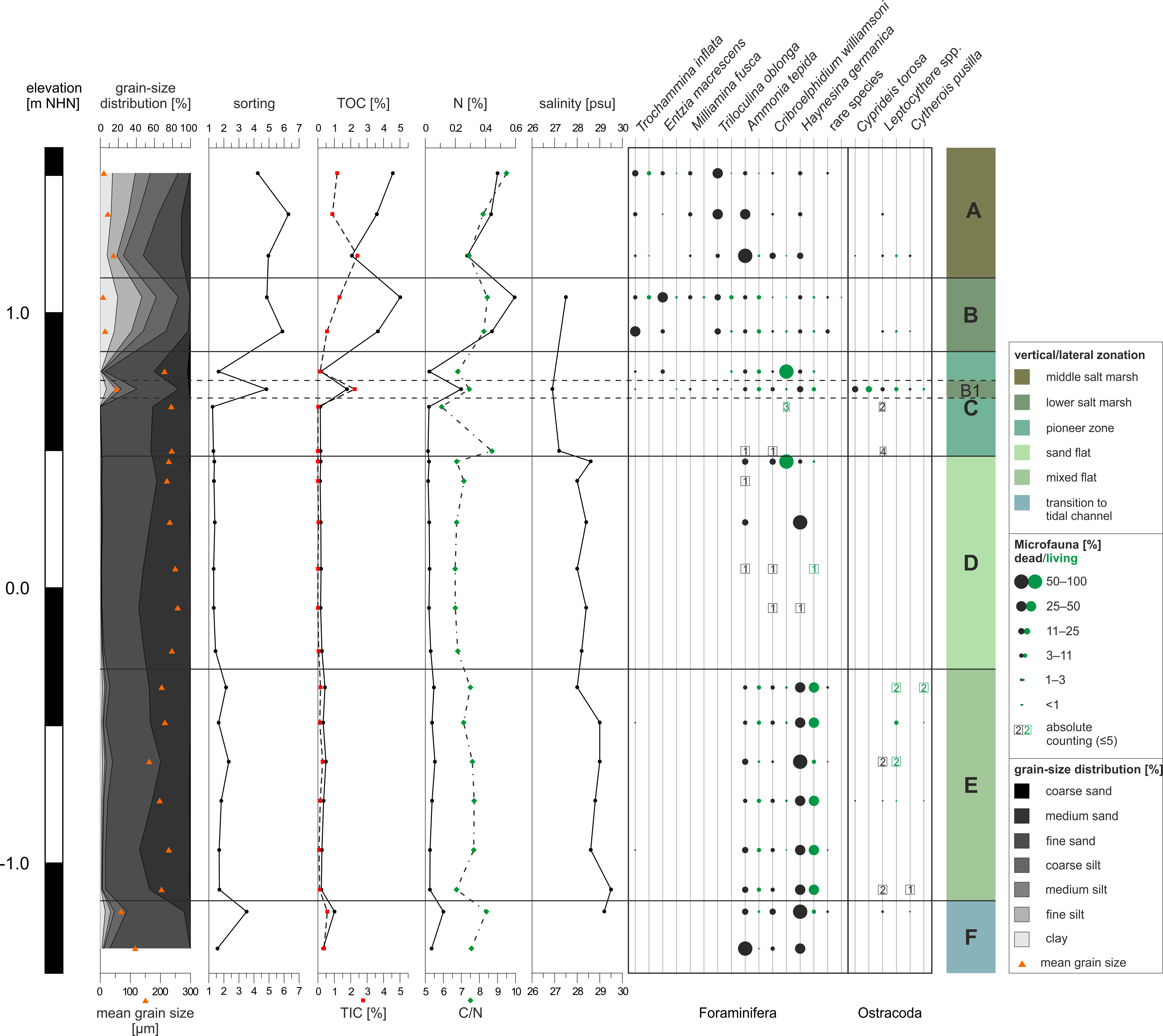
Figure 4. Microfaunal, sedimentological and geochemical results of the investigated surface transect in relation to the elevation. From left to right: grain-size distribution and mean grain size; sorting of the sediments, content of organic (TOC) and inorganic (TIC) carbon; nitrogen (N) content and ratio of organic carbon and nitrogen (C/N); salinity trend measured for sampling points with present water coverage; foraminifer and ostracod species association; identified lateral and vertical zones.
17Zone B (lower salt marsh), comprising three adjacent samples (c. 1.06–0.86 m NHN; samples 4, 5 and 6), is characterised by very poorly sorted sandy mud with an increasing sand amount towards lower elevations. The vegetation is composed of Atriplex portulacoides (salt bush), Puccinellia maritima (andel grass) and Spartina anglica (cord grass). The highest TOC and second highest TIC values of the whole transect occur in this zone as well as the highest values for N. Water coverage is partially given by small pools near the sampling points with a salinity of 27.5 psu in the upper part of Zone B. This zone, with abundances of up to c. 600 individuals/10 cm³, is further defined by the presence of T. inflata, E. macrescens and M. fusca. E. macrescens dominates the upper part (sample 20), while T. inflata dominates the lower part (sample 5), both followed by the hyaline foraminifer species T. oblonga, A. tepida, H. germanica and C. williamsoni. Ostracods are only present in the lower part of the zone, dominated by Leptocythere and accompanied by C. pusilla. Only ~11–22% of all present foraminifers, but half of the ostracods were identified as ‘living’. However, compared to the amount of foraminifers, ostracods only show very low abundances. Sample 5 taken from a small salt-marsh pool (0.72 m NHN, laterally belonging to the lower salt marsh) stands out in Zone B and represents Subzone B1. It is characterised by a much higher sand amount (sandy mud), higher TIC, lower TOC and N values as well as a lower C/N ratio than in the rest of Zone B. The salinity also decreases to the lowest value of the complete transect. The microfaunal composition changes in this subzone with a slightly higher amount of living Foraminifera (~25%). Foraminifera are dominated by H. germanica followed by A. tepida and C. williamsoni, accompanied by only a few individuals of T. oblonga and only one specimen of T. inflata. Ostracoda are strongly dominated by dead (~25%) and living (~43%) individuals of C. torosa, accompanied by Leptocythere and C. pusilla. This sample shows the highest amount of ostracods throughout the complete transect. Within the complete zone (including B1), the microfaunal concentration decreases towards Zone C from c. 500 ind./10 cm³ to c. 100 ind./10 cm³. Only very few shells seem slightly degraded, whereas the major part is well preserved.
18Zone C (pioneer zone; c. 0.86–0.48 m NHN) comprises three samples (7, 8 and 9) and represents a transition to Zone D, i.e. a transition from the salt marsh to the tidal flat. It is characterised by moderately to well sorted sand. Spartina anglica (cord grass) dominates the vegetation of this zone. No TIC and almost no TOC and N were documented. The C/N ratio first decreases before increasing to the highest value throughout the transect in the last sample of this zone. Water coverage in this zone occurred mainly in the lower part, which is the border between salt marsh and sand flat, due to the neap tide situation at the sampling day in 2015. The salinity is higher than in Zone B. The amount of microfauna (mainly foraminifers) is much lower than in Zone B, even though the uppermost sample still shows a moderate concentration of individuals. It is strongly dominated (62%) by living individuals of C. williamsoni followed by H. germanica and A. tepida accompanied by only one individual each of T. inflata and T. oblonga. In terms of Ostracoda, only six individuals of Leptocythere occurred in the lower two samples. The microfaunal concentration strongly decreases with decreasing elevation with c. 120 ind./10 cm³ in the upper sample (7) and only 4–6 ind./10 cm³ in the lower two samples. Most of the shells are well preserved and only very few seem slightly degraded.
19Zone D (sand flat; c. 0.48–-0.30 m NHN) comprises six samples (10–15) and is the widest zone of the transect with a length of ~750 m. It is characterised by moderately well to well sorted sand with a coarsening trend towards lower elevations (medium sand increasing from c. 40 to c. 52%, fine sand decreasing from c. 51 to 38%). No vegetation was present in 2015 (winter), while occasional carpets of algae characterised the zone in 2017 (summer). TIC values are negligible as well as the only slightly higher TOC and N values. The C/N ratio is at a quite constant level (6–7). Water coverage occurred in the form of small puddles or micro-channels in a higher number in 2015 than in 2017. All samples are situated within these water-covered areas. The salinity shows only slight variations (0.6 psu). There are very few foraminifers in this zone (0–30 ind./10 cm³), dominated by living C. williamsoni in the upper part, where A. tepida is also present, and by dead H. germanica in the central part. The lower part of the zone comprises even fewer individuals while ostracods are completely absent. The few foraminifers observed in this zone show signs of degradation, except for the living individuals of C. williamsoni, which are well preserved.
20In Zone E (mixed flat; c. -0.30–-1.14 m NHN), comprising six samples (16–21), silt and clay reappear (Fig. 4). It is characterised by a poorly to moderately sorted muddy sand to pure sand. No vegetation is present. In this zone, for the first time, occasional molluscs induce slight bioturbation of the upper centimetres of the sediment. TIC, TOC, N and the C/N ratio show slight variations compared to Zone D. Water coverage occurred in the form of small puddles or micro-channels and the salinity increases from the upper to the lower part by 1.5 psu, resulting in the highest value of the transect (29.5 psu). Besides the grain-size distribution, the most striking change is the reappearance of microfauna with generally increasing concentrations towards lower elevations (from c. 50 to c. 900 ind./10 cm³). It is dominated by H. germanica (living and dead) followed by A. tepida, C. williamsoni and two individuals of T. inflata. The highest abundance of ostracods (20 individuals) occurs in sample 17 dominated by living Leptocythere (like in the rest of Zone E). While C. pusilla and C. torosa are also present, some juvenile ostracod individuals remain indeterminable (8 out of 49 in total). Preservation of shells is mainly good and only very few individuals seem slightly degraded.
21Zone F (transition to tidal channel; c. -1.14 m NHN until at least -1.31 m NHN) comprises two samples (22 and 23). With first increasing and then decreasing silt and clay amounts, it is characterised by poorly to moderately sorted muddy sand. In 2015, no vegetation was present, while in 2017 algae remains were visible along the levee of the tidal channel. Furthermore, the levee was characterised by many mollusc shells (Fig. 2d). In the upper sample, TIC, TOC and N show a slight increase of 0.09–0.8%, while the C/N ratio increases by ~1.6 and only the salinity shows a slight decrease of 0.3 psu. In the lower sample 23, all values are more similar to Zone E. Due to the lack of water cover, no salinity was measured for the lowest sample, but the salinity of the shallow water of the adjacent tidal channel was 29.3 psu. The foraminiferal composition is similar to that of Zone E, although the amount of living individuals decreases with decreasing elevation, as does the microfaunal concentration (from c. 2500 to c. 1000 ind./10 cm³). Towards the lowermost sample (23), a shift in the dominance between the two most abundant tidal flat foraminifer species of the transect – H. germanica and A. tepida – is observed; C. williamsoni occurs as well. Ostracods are only present in the upper sample represented by dead Leptocythere and C. pusilla. Approximately half of the shells or tests are well preserved, while the rest appears to be slightly degraded.
22Plate 1. SEM images of frequently documented foraminifer (1–11) and ostracod (12–15) species. 1, 2: Ammonia tepida (Cushman, 1926); 3, 4: Haynesina germanica (Ehrenberg, 1840); 5, 6: Cribroelphidium williamsoni (Haynes, 1973); 7: Triloculina oblonga (Montagu, 1803); 8, 9: Entzia macrescens (Brady, 1870); 10: Trochammina inflata (Montagu, 1803); 11: Miliammina fusca (Brady, 1870); 12: Cytherois pusilla (Sars, 1928); 13: Leptocythere pellucida (Baird, 1850); 14, 15: Cyprideis torosa (Jones, 1850).
5. Results of statistical analyses
5.1. Driving environmental factors
23The Pearson correlation shows that T. oblonga is highly correlated with the sand amount, N and TOC (and these factors are also highly correlated with each other). The sand amount and the N content were therefore excluded for the downstream statistical analyses. Since TIC seems to be rather insignificant throughout the transect and TOC is also connected to the grain size, we also excluded TIC for the multivariate statistics. Furthermore, Spirillina sp. is highly correlated with M. fusca, the latter being slightly more frequent. Therefore, the rare Spirillina sp. was also excluded. In order to find variables, which account for as much of the variance in our dataset as possible (Davis, 1986; Harper, 1999), a principle component analysis (PCA) was performed. In order to receive statistically relevant results, only samples with a minimum of 40 individuals counted were considered, thus excluding almost all sand flat samples between c. 0.39 and -0.29 m NHN. The most relevant axes for our modern dataset are PC 1 and 2 (biplot in Fig. 5).
Figure 5. PCA biplots of the investigated surface transect with identified groupings (for colour legend of facies zones see fig. 3). Black diamonds represent samples (two outliers marked in yellow), blue diamonds represent microfaunal taxa.
24PC 1, with an explained variance of 53.48%, contrasts T. oblonga and C. williamsoni along with all agglutinated foraminifer species with H. germanica. This includes all salt marsh and transitional samples on the negative and all tidal flat samples on the positive side leading to the conclusion of PC 1 describing a ‘salt marsh versus tidal flat’ factor, which could be related to the duration of water cover, i.e. the elevation. PC 2, describing a variance of 26.09%, opposes mainly T. oblonga (associated with the salt marsh samples) and C. williamsoni (associated with the transitional samples of the pioneer zone and sand flat). Since C. williamsoni tolerates higher salinities than most salt marsh species (Murray, 2006), PC 2 could relate to the salinity, which does not seem to have much of an influence on the tidal flat samples. The two samples of Zone F (transition to the tidal channel; samples 22 and 23 marked in yellow in Fig. 5) seem to be ‘misplaced’ by the PCA, since sample 22 is associated with the tidal flat group, whereas sample 23 is situated at the ‘salt marsh’ side of PC 1 and associated to A. tepida. This may be explained by the position at the margin of the tidal channel and related higher-dynamic conditions, to which A. tepida seems to be better adapted.
25As shown by the PCA, the elevation seems to have a strong influence on foraminifer and ostracod distribution. In order to test if it is the main driving environmental factor, a canonical correspondence analysis (CCA) was carried out including the microfaunal data and the remaining parameters elevation, TOC and C/N. The CCA biplot (Fig. 6) shows the first axis, describing a variance of 63.73%, with highest scores for TOC and elevation (in ranking order). The latter exhibits the highest score for the second axis, which describes a variance of 28.52%. The C/N ratio seems rather irrelevant for both axes with the lowest scores for both. The different species exhibit different relations to the depicted environmental parameters. Since the second axis is mainly described by the elevation, the foraminifer species A. tepida and C. williamsoni and all three ostracod species show the highest relation to this parameter, whereas the salt marsh foraminifers T. oblonga, M. fusca and T. inflata are highly related to TOC, mainly describing the first axis. This indicates that the foraminifer and ostracod distribution is mainly influenced by the organic content and the inundation frequency related to elevation. Since the elevation is related to both axes and the TOC content shows quite high correlation values concerning the elevation (~0.75), a strong influence of the elevation, related to water depth and inundation frequency, can be assumed.
Figure 6. CCA biplot of the investigated surface transect. Black diamonds represent samples, blue diamonds represent microfaunal taxa. The three remaining environmental factors (elevation, TOC and C/N) are visualised by green lines. TOC and elevation have the highest scores for axes 1 and 2, identifying them as the main influence on the dataset.
26A detrended correspondence analysis (DCA) was carried out in order to test the species-environment relationship. Since PCA and CCA confirmed the elevation (i.e. inundation frequency) as the strongest driving factor, we included only the elevation and the microfaunal data for the DCA. As the DCA plot (Fig. 7) shows, the length of the environmental gradient was determined as 3.3 SD, which indicates a rather unimodal species response (e.g. Birks, 1995; Lepš & Šmilauer, 2003).
Figure 7. DCA plot showing the length of the environmental gradient (x=330, i.e. 3.3 pointing to unimodal species distributions). Samples are represented by black, species by blue diamonds.
5.2. Transfer function (TF) development and testing
27Since living associations of foraminifers and ostracods can be affected by seasonal differences and the 2015 and 2017 samples were taken during different seasons – in fact showing differences in the densities of living individuals (Fig. 4) – only the dead assemblages were used for the TF development. Those represent the result of habitat preferences and connected taphonomic changes averaged over several years (e.g. Murray, 2000).
28Two different models were developed for the TF (Fig. 8): Model I using exclusively foraminifers, representing the most commonly applied procedure, and Model II including the ostracods. Again, only samples with a minimum of 40 individuals were considered. For both models, component 2 seems to be the most suitable (lowest RMSEP and highest R²) and is presented here. Since during the initial modelling, sample 23, once again, turned out to be an outlier, it was excluded from the dataset reducing the investigated elevation gradient to a vertical distance of 2.69 m (+1.51 to -1.18 m NHN). Since samples were taken during different tidal situations (neap and spring tide), the description of the RMSEP is related to the mean tidal range instead of the mean spring tidal range.
29Model I shows an R²boot of 0.82 and an RMSEP of 54.2 cm, which accounts for 20.2% of the elevation gradient (and 20.1% of the mean tidal range). There is no visible trend of the TF over- or underestimating samples in relation to their observed elevation and structures of residuals are also not noticeable (Fig. 8).
30Model II shows a slightly better R²boot of 0.84 and with 49.1 cm also a better RMSEP accounting for only 18.3% of the total elevation gradient (and 18.2% of the mean tidal range). Again, there is neither a clear trend of over- or underestimation related to the observed elevation nor are there visible structures of the residuals (Fig. 8).
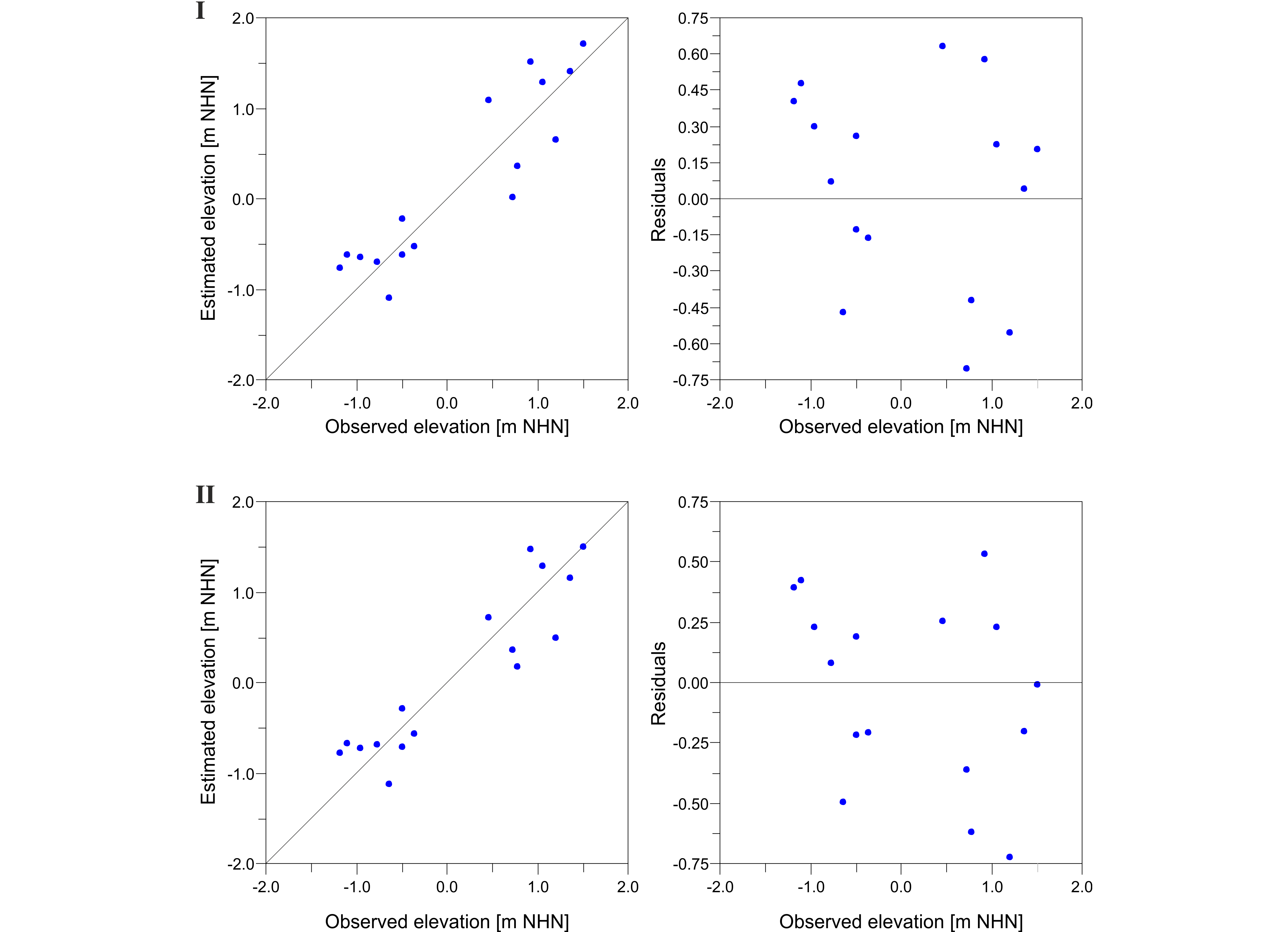
Figure 8. Results of testing the transfer function (TF) by bootstrapping cross validation (1000 cycles). Diagrams depict estimated vs. observed elevation (left diagrams) and deviation of each sample from the observed elevation (right diagrams) for both Model I based on dead Foraminifera alone (top) and Model II based on dead Foraminifera and Ostracoda combined (bottom).
6. Discussion and evaluation of the modern training set
6.1. General observations
31In general, higher amounts of fine-grained sediments, TIC, TOC and N correlate very well with the presence of microfauna, whereas areas of coarser-grained sediments and constantly low TIC, TOC and N contents correspond to areas of low abundance or even complete absence. The C/N ratio, lying between 4 and 10 throughout the complete transect, indicates that all organic matter originates from aquatic sources (e.g. Last & Smol, 2001). In accordance with our expectations, the salinity shows a general rising trend from the salt marsh to the tidal channel and increasing water cover and depths (Kaiser & Niemeyer, 1999; Flöser et al., 2011).
6.2. Living vs. dead fauna
32Comparing the living and dead associations, we notice differences along the transect. The remarkably lower percentages of living than dead individuals occurring in the middle salt marsh (Zone A) suggest a quite good preservation of tests without significant dissolution effects. Furthermore, a part of the observed foraminifers and ostracods could be allochthonous and introduced during spring tides or storm surges (cf. de Rijk & Troelstra, 1999).
33In the lower salt marsh (Zone B), especially in the salt-marsh pool (Subzone B1), the discrepancy between living and dead individuals is smaller, indicating either a poorer preservation of empty tests or better living conditions, mostly due to the higher frequency of water coverage at this elevation. Moreover, the permanently covered salt-marsh pool provides good living conditions with new, probably oxygen-rich water inundating during high tide and provided by rainfall combined with bioturbation (roots) and diffusion (cf. de Rijk & Troelstra, 1999; Berkeley et al., 2007). Furthermore, its surrounding is sheltered by the vegetation of the lower salt marsh enabling permanent water coverage, which results in the quite high number of living foraminifers and ostracods, especially C. torosa (e.g. Athersuch et al., 1989; Murray, 2006). Probably, a combination of better living conditions (higher numbers of living individuals) and poorer preservation led to the observations for this zone.
34In the pioneer zone (Zone C), a clear dominance of living C. williamsoni is observed, whereas the dead fauna is more diverse. Since C. williamsoni prefers sediments with <60% mud/silt content (Murray, 2006), this pattern correlates well with the abruptly increased sand amount in this zone, also reflecting the higher dynamics in the transition area between salt marsh and tidal flat (Nyandwi & Flemming, 1995). Due to a higher energy level, dead individuals could, once again, be introduced by the tidal current. The situation is similar in the upper part of the sand flat (Zone D), where the transition sample again is strongly dominated by living C. williamsoni. However, since the rest of the sand flat shows only one living and a few dead individuals, dynamics seem to get too intense towards the lower parts of the sand flat for the survival of foraminifers or tests underlie post-mortem removal by currents (Hofker, 1977). Another reason for the very low occurrence of microfauna may be the very low (organic and inorganic) carbon content in the sand flat. Processes of early diagenesis (Berkeley et al., 2007) could influence the test preservation through changed saturation rates of calcium carbonate (CaCO3) causing the dissolution of tests (Sanders, 2003).
35A completely different situation is documented in the mixed flat (Zone E). Foraminifers show a similar pattern in both living and dead associations indicating a good fossilisation potential (cf. Smith, 1987). Ostracods show higher abundances of living individuals in the upper part and of dead ones in the lower part suggesting that they experience post-mortem transport towards the tidal channel (e.g. Edwards & Horton, 2000; Frenzel & Boomer, 2005). In the transition area to the tidal channel (Zone F), living individuals are very few compared to dead ones, which may be due to the current of the channel complicating the settlement of foraminifers as well as ostracods (e.g. Hofker, 1977; Murray, 2006). However, since dead shells are easier to be carried away by the current, this could again suggest a very good preservation of empty tests. Still, it needs to be taken into account that a certain part of the observed dead individuals is probably introduced by the tidal current. The few dead ostracods could have been transported from the adjacent mixed flat.
6.3. Evaluation of the transfer function (TF)
36Adding the ostracod data to our training set improves sea-level estimations for the higher elevation stations only. The reason for this result is the higher abundance of ostracods in these samples from the tidal pond and surroundings. Thus, more detailed data would likely improve the performance of the TF. We would expect a similar outcome for the deeper stations as well but this needs samples with higher ostracod counts, a target for future studies.
37Although the inclusion of ostracods clearly improves the TF performance and an RMSEP of 18.3% seems acceptable (Barlow et al., 2013), a vertical error of ~49 cm, leading to a total error range of the indicative meaning of ~1 m, is still comparably large (Edwards & Wright, 2015). Since other studies of similar environments focus only on the vegetated marsh (e.g. Edwards & Horton, 2000; Gehrels & Newman, 2004; Kemp et al., 2013; Müller-Navarra et al., 2017), the relatively high vertical error could be related to the high environmental gradient (2.69 m; approx. the mean tidal range of Spiekeroog). However, the tidal flat needs to be included in the TF, since the sediment cores dedicated to the future TF application cover large sections of tidal flat and salt marsh deposits. In general, it has to be noted that the exclusion of the sand-flat samples with <40 individuals leads to a lack of information about estimates within the elevation range of these samples (from 0.39 to -0.29 m NHN), which may lead to a deteriorated predictive ability for equivalent palaeo-elevations. We expect that a higher number of training samples will result in a better TF performance as most studies base their TF on a minimum of 40 samples, resulting in smaller error ranges (e.g. Kemp et al., 2012; Müller-Navarra et al., 2016, 2017; Milker et al., 2017). In a next step we will, therefore, increase the total number of samples in order to fill the elevation gap created by the weak sand flat samples.
6.4. Transfer function (TF) vs. peat-based reconstruction
38The vertical error range (~1 m) of Model II of our TF is significantly smaller than the one of existing peat-based RSL reconstructions of up to 3–5 m (e.g. Long et al., 2006; Bungenstock & Schäfer, 2009; Bungenstock & Weerts, 2010, 2012; Baeteman et al., 2011). Reasons for the better performance of the TF include:
39The TF provides a direct relation to the sea level, whereas peat has an indirect relation to the sea level. However, the indicative meaning of peat is still not universally defined (e.g. Baeteman, 1999; van de Plassche et al., 2005; Bungenstock & Schäfer, 2009; Wolters et al., 2010). Moreover, basal peat cannot always be used as sea-level index point. For example, for the early Holocene, Wolters et al. (2010) document a basal peat, which cannot be linked to sea level, as sea level was ~17 m lower, when peat growth started. They state that sea level-independent paludification in special topographic conditions is well known as described by e.g. Jelgersma, 1961; Lange & Menke, 1967; Baeteman, 1999. However, widespread intercalated peat layers are, in general, used as RSL index points, but close investigation of formation processes is essential (Bungenstock & Schäfer, 2009; Bungenstock & Weerts, 2010).
40Post-depositional compaction results in high uncertainty for peat-based RSL reconstructions and significantly affects intercalated peats and the upper parts of basal peats. Horton & Shennan (2009) found average compaction rates of 0.4±0.3 mm/yr for peats buried in Holocene sequences along the east coast of England. The TF, however, can be applied to a wide range of intertidal facies and sequences comprising large amounts of compaction-prone peat can be avoided.
41The microfossil-based TF also helps to avoid uncertainties imposed by relocated peat, which is ripped off at peat cliffs in so-called ‘Dargen’ and transported over wide areas (e.g., Pliny the Elder (Naturalis Historia, XVI, 5-6) in Herrmann, 1988; Streif, 1990; Behre & Kučan, 1999; van Dijk et al., 2019) potentially resulting in age inversions in Holocene stratigraphies and invalid RSL indication.
42Finally, the microfossil-based TF is a promising tool to derive RSL information from the uppermost part of the Holocene sequence in the wider region covering the last 2000 years, where peats are usually rare.
6.5. Method evaluation
43As a few additional samples were taken during the summer, whereas the main transect was sampled during winter time, differences in the living microfauna between these samples could be well explained by seasonal differences. However, since only dead individuals were used for the TF development, in order to capture information over a longer time period (Murray, 2000), this is not expected to influence the outcome of our study.
44Concerning the sampling thickness, most studies dealing with microfaunal surface distributions only use the uppermost 1 cm of the surface sediments (e.g. Kemp et al., 2012; Korsun et al., 2014; Shaw et al., 2016; Müller-Navarra et al., 2016, 2017). However, due to the high dynamics in the meso-tidal Wadden Sea and expected infaunal foraminifer taxa down to a depth of up to 5 cm (Hofker, 1977), we decided for deeper sampling. By investigating down to a depth of 3 cm, we account for most of the potential habitats of living individuals in order to better represent the modern conditions in our analysis. Given the dm-scale accuracy of the TF, the error imposed by the vertical integration of 3 cm is negligible for future RSL reconstructions. This sampling depth will, however, require undisturbed fossil inter- and supratidal layers with a minimum thickness of 3 cm for the future application of the TF.
45Many of the studies applying Foraminifera to sea-level problems pick the individuals wet in order to prevent drying of organic components and potential damaging of agglutinated taxa (e.g. de Rijk, 1995; Edwards & Wright, 2015; Milker et al., 2016; Müller-Navarra et al., 2016, 2017), whereas in the present study most of the samples were picked dry. However, since we did not observe any significant effects of drying on species associations or preservation of agglutinated taxa, which is similar to observations of, e.g., Schönfeld et al. (2013), we assess our results to be comparable with those of previous studies.
7. Conclusion and outlook
46The investigated surface transect in the back-barrier salt marsh and tidal flat of the island of Spiekeroog shows a clear vertical as well as lateral zonation of both foraminifers and ostracods. While environmental factors like the hydro-energetic level (reflected by grain-size distribution), the food availability (organic carbon) and the CaCO3 saturation (inorganic carbon) influence this zonation, the major influence is given through the water depth or the duration of water cover (connected to the elevation). Hence, our surface transect shows a good potential for the establishment of a relative sea-level transfer function (RSL TF). The common TF model, using only dead foraminifer associations, was improved by ~5 cm (vertical error), resulting in an improvement of the error range of ~10 cm, by including dead ostracod associations. The improved TF provides an R²Boot of 0.84 and a vertical error of 49.1 cm accounting for 18.3% of the investigated elevation gradient of ~2.7 m, which is the approximate tidal range of Spiekeroog (BSH, 2018). Even though this vertical error is already lower than the one associated with previously used RSL index points such as basal or intercalated peats, a clear demand for higher resolutions and lower error ranges remains (e.g. Vink et al., 2007; Bungenstock & Schäfer, 2009; Bungenstock & Weerts, 2010, 2012; Baeteman et al., 2011). Thus, further improvements of our TF will be attempted in the near future by integrating additional modern local samples in order to expand the modern training set. Further improvements could probably be accomplished by narrowing the environmental gradient or by combining the dataset with existing data from North Frisia collected by Müller-Navarra et al. (2017) in order to develop a regional TF. In a final step, the RSL TF will be applied to Holocene sedimentary records already recovered by the WASA (Wadden Sea Archive) project (Bittmann, 2019).
8. Acknowledgements
47The research reported here is part of the WASA project (The Wadden Sea as an archive of landscape evolution, climate change and settlement history: exploration – analysis – predictive modelling) funded by the “Niedersächsisches Vorab” of the VolkswagenStiftung within the funding initiative “Küsten und Meeresforschung in Niedersachsen” of the Ministry for Science and Culture of Lower Saxony, Germany (project VW ZN3197). We gratefully acknowledge Dr. Yvonne Milker (University of Hamburg) for her help regarding statistical analyses and interpretations. The head of the WASA project, Dr. Felix Bittmann (Lower Saxony Institute for Historical Coastal Research), is acknowledged for proofreading and valuable comments on the manuscript. We also appreciate the very constructive and helpful comments by Dr. Simon Engelhart and one anonymous reviewer. Sampling and analyses of most of the samples were carried out during the funding period of the Start-up Honours Grant 2016A of the Graduate School of Geosciences, University of Cologne, awarded to J.S. This research is a contribution to IGCP Project 639 ‘Sea Level Change from Minutes to Millennia’.
9. References
48Athersuch, J., Horne, D.J. & Whittaker, J.E., 1989. Marine and brackish water ostracods (superfamilies Cypridacea and Cytheracea): keys and notes for the identification of the species. Brill, Leiden, Synopses of the British fauna, 43, 343 p.
49Baeteman, C., 1999. The Holocene depositional history if the Ijzer palaeo-valley (western Belgian coastal plain) with reference to the factors controlling the formation of intercalated peat beds. Geologica Belgica, 2, 39–72.
50Baeteman, C., Waller, M. & Kiden, P., 2011. Reconstructing middle to late Holocene sea‐level change: A methodological review with particular reference to ‘A new Holocene sea‐level curve for the southern North Sea’ presented by K.‐E. Behre. Boreas, 40, 557–572. https://doi.org/10.1111/j.1502-3885.2011.00207.x
51Barlow, N.L.M., Shennan, I., Long, A.J., Gehrels, W.R., Saher, M.H., Woodroffe, S.A. & Hiller, C., 2013. Salt marshes as late Holocene tide gauges. Global and Planetary Change, 106, 90–110. https://doi.org/10.1016/j.gloplacha.2013.03.003
52Beck, H.E., Zimmermann, N.E., McVicar, T.R., Vergopolan, N., Berg, A. & Wood, E.F., 2018. Present and future Köppen-Geiger climate classification maps at 1-km resolution. Scientific Data, 5, 180214. https://doi.org/10.1038/sdata.2018.214
53Beets, D.J. & Van der Spek, A.J.F., 2000. The Holocene evolution of the barrier and the back-barrier basins of Belgium and The Netherlands as a function of late Weichselian morphology, relative sea-level rise and sediment supply. Netherlands Journal of Geosciences, 79(1), 3–16. https://doi.org/10.1017/S0016774600021533
54Behre, K.-E., 1987. Meeresspiegelbewegungen und Siedlungsgeschichte in den Nordseemarschen. Holzberg-Verlag, Oldenburg, Vorträge der Oldenburgischen Landschaft, 17, 47 p.
55Behre, K.-E., 2007. A new Holocene sea-level curve for the southern North Sea. Boreas, 36, 82–102. https://doi.org/10.1080/03009480600923386
56Behre, K.-E. & Kučan, D., 1999. Neue Untersuchungen am Außendeichsmoor bei Sehestedt am Jadebusen. Probleme der Küstenforschung im südlichen Nordseegebiet, 26, 35–64.
57Behre, K.-E. & Streif, H., 1980. Kriterien zu Meeresspiegel- und darauf bezogene Grundwasserabsenkungen. E&G Quaternary Science Journal, 30, 153–160. https://doi.org/10.3285/eg.30.1.12
58Berkeley, A., Perry, C.T., Smithers, S.G., Horton, B.P. & Taylor, K.G., 2007. A review of the ecological and taphonomic controls on foraminiferal assemblage development in intertidal environments. Earth-Science Reviews, 83, 205–230. https://doi.org/10.1016/j.earscirev.2007.04.003
59Birks, H.J.B., 1995. Quantitative palaeoenvironmental reconstructions. In Maddy, D. & Brew, J.S. (eds), Statistical Modelling of Quaternary Science Data. Quarternary Research Association, Cambridge, Technical Guide 5. 161–254.
60Bittmann, F., 2019. Das Wattenmeer als Archiv zur Landschaftsentwicklung, Klimaänderung und Siedlungsgeschichte. Nachrichten des Marschenrats zur Förderung der Forschung im Küstengebiet der Nordsee, 56, 25–27.
61Blott, S.J. & Pye, K., 2001. Gradistat: A grain size distribution and statistics package for the analysis of unconsolidated sediments. Earth Surface Processes and Landforms, 26, 1237–1248. https://doi.org/10.1002/esp.261
62Bundesamt für Seeschifffahrt und Hydrographie (BSH), 2018. Gezeitenkalender 2018: Hoch- und Niedrigwasserzeiten für die Deutsche Bucht und deren Flussgebiete. Bundesamt für Seeschifffahrt und Hydrographie, Hamburg, 136 p.
63Bungenstock, F. & Schäfer, A., 2009. The Holocene relative sea-level curve for the tidal basin of the barrier island Langeoog, German Bight, Southern North Sea. Global and Planetary Change, 33, 34–51. https://doi.org/10.1016/j.gloplacha.2008.07.007
64Bungenstock, F. & Weerts, H.J.T., 2010. The high-resolution Holocene sea-level curve for Northwest Germany: global signals, local effects or data-artefacts? International Journal of Earth Sciences, 99, 1687–1706. https://doi.org/10.1007/s00531-009-0493-6
65Bungenstock, F. & Weerts, H.J.T., 2012. Holocene relative sea-level curves for the German North Sea coast. International Journal of Earth Sciences, 101, 1083–1090. https://doi.org/10.1007/s00531-011-0698-3
66Bungenstock, F., Wehrmann, A., Hertweck, G. & Schäfer, A., 2002. Modification of current systems and bedforms during the tidal cycle on tidal flats of the barrier island Baltrum, Southern North Sea. Zentralblatt für Geologie und Paläontologie, Teil I, 2001, 283–295.
67Davis, J.C., 1986. Statistics and Data Analysis in Geology. John Wiley & Sons, New York, 656 p.
68de Rijk, S., 1995. Salinity control on the distribution of salt marsh foraminifera (Great Marshes, Massachusetts). Journal of Foraminiferal Research, 25, 156–166. https://doi.org/10.2113/gsjfr.25.2.156
69de Rijk, S. & Troelstra, S., 1999. The application of a foraminiferal actuo-facies model to salt-marsh cores. Palaeogeography, Palaeoclimatology, Palaeoecology, 149, 59–66. https://doi.org/10.1016/S0031-0182(98)00192-8
70Edwards, R.J. & Horton, B.P., 2000. Reconstructing relative sea-level change using UK salt-marsh foraminifera. Marine Geology, 169, 41–56. https://doi.org/10.1016/S0025-3227(00)00078-5
71Edwards, R. & Wright, A., 2015. Foraminifera. In Shennan, I., Long, A.J. & Horton, B.P. (eds), Handbook of Sea-Level Research. AGU/Wiley, Hoboken, 191–217. https://doi.org/10.1002/9781118452547.ch13
72Engelhart, S.E. & Horton, B.P., 2012. Holocene sea level database for the Atlantic coast of the United States. Quaternary Science Reviews, 54, 12–25. https://doi.org/10.1016/j.quascirev.2011.09.013
73Eshel, G., Levy, G.J., Mingelgrin, U. & Singer, M.J., 2004. Critical evaluation of the use of laser diffraction for particle-size distribution analysis. Soil Science Society of America Journal, 68, 736–743. https://doi.org/10.2136/sssaj2004.7360
74Filipescu, S. & Kaminski, M.A., 2011. Re-discovering Entzia, an agglutinated foraminifer from the Transylvanian salt marshes. In Kaminski, M.A. & Filipescu, S. (eds), Proceedings of the Eighth International Workshop on Agglutinated Foraminifera. Grzybowski Foundation Special Publication, 16, 29–35.
75Flemming, B.W., 2002. Effects of climate and human interventions on the evolution of the Wadden Sea depositional system (southern North Sea). In Wefer, G., Berger, W., Behre, K.-E. & Janssen, E. (eds), Climate Development and History of the North Atlantic Realm. Springer, Berlin, 399–413. https://doi.org/10.1007/978-3-662-04965-5_26
76Flöser, G., Burchard, H. & Riethmüller, R., 2011. Observational evidence for estuarine circulation in the German Wadden Sea. Continental Shelf Research, 31, 1633–1639. https://doi.org/10.1016/j.csr.2011.03.014
77Folk, R.L. & Ward ,W.C., 1957. Brazos River Bar: a study in the significance of grain size parameters. Journal of Sedimentary Research, 27, 3–26. https://doi.org/10.1306/74D70646-2B21-11D7-8648000102C1865D
78Frenzel, P. & Boomer, I., 2005. The use of ostracods from marginal marine, brackish waters as bioindicators of modern and Quaternary environmental change. Palaeogeography, Palaeoclimatology, Palaeoecology, 225, 68–92. https://doi.org/10.1016/j.palaeo.2004.02.051
79Frenzel, P., Keyser, D. & Viehberg, F.A., 2010. An illustrated key and (palaeo) ecological primer for Postglacial to Recent Ostracoda (Crustacea) of the Baltic Sea. Boreas, 39/3, 567–575. https://doi.org/10.1111/j.1502-3885.2009.00135.x
80Freund, H. & Streif, H., 1999. Natürliche Pegelmarken für Meeresspiegelschwankungen der letzten 2000 Jahre im Bereich der Insel Juist. Petermanns Geographische Mitteilungen, 143, 34–45.
81Freund, H. & Streif, H., 2000. Natural sea-level indicators recording the fluctuations of the mean high tide level in the southern North Sea. Wadden Sea Newsletter, 2, 16–18.
82Gehrels, W. R. & Newman, S.W., 2004. Salt-marsh foraminifera in Ho Bugt, western Denmark, and their use as sea-level indicators. Geografisk Tidsskrift – Danish Journal of Geography, 104/1, 97–106. https://doi.org/10.1080/00167223.2004.10649507
83Gehrels, W.R., Belknap, D.F., Black, S. & Newnham, R.M., 2002. Rapid sea-level rise in the Gulf of Maine, USA, since AD 1800. The Holocene, 12/4, 383–389. https://doi.org/10.1191/0959683602hl555ft
84Gerlach, A., 1999. Pflanzengesellschaften auf Spülsäumen. In Henke, S., Roy, M. & Andrae, C. (eds), Umweltatlas Wattenmeer. Band 2, Wattenmeer zwischen Elb- und Emsmündung. Ulmer, Stuttgart, 58–59.
85Hammer, Ø., Harper, D.A.T. & Ryan, P.D, 2001. PAST: Palaeontological statistics software package for education and data analysis. Palaeontologica Electronica, 4/1, article 4.
86Harper, D.A.T. (ed.), 1999. Numerical Palaeobiology. John Wiley & Sons, Chichester, 468 p.
87Herrmann, J. (ed.), 1988. Griechische und lateinische Quellen zur Frühgeschichte Mitteleuropas bis zur Mitte des 1. Jahrtausends u.Z. 1, von Homer bis Plutarch. Akademie Verlag, Berlin, 657 p.
88Hofker, J., 1977. The foraminifera of Dutch tidal flats and salt marshes. Netherlands Journal of Sea Research, 11, 223–296. https://doi.org/10.1016/0077-7579(77)90009-6
89Horton, B.P & Edwards, R.J, 2006. Quantifying Holocene Sea Level Chance Using Intertidal Foraminifera: Lessons from the British Isles. Cushman Foundation for Foraminiferal Research, Special Publication, 40, 97 p.
90Horton, B.P. & Shennan, I., 2009. Compaction of Holocene strata and the implications for relative sea-level change on the east coast of England. Geology, 37, 1083–1086. https://doi.org/10.1130/G30042A.1
91Jelgersma, S., 1961. Holocene sea level changes in the Netherlands. Mededelingen van de Geologische Stichting, C(7), 1–100.
92Juggins, S., 2007. C2 Version 1.5: software for ecological and palaeoecological data analysis and visualisation. University of Newcastle, Newcastle upon Tyne.
93Kaiser, R. & Niemeyer, H.D., 1999. Wasser-Beschaffenheit. In Henke, S., Roy, M. & Andrae, C. (eds), Umweltatlas Wattenmeer. Band 2, Wattenmeer zwischen Elb- und Emsmündung. Ulmer, Stuttgart, 32–33.
94Kemp, A.C. & Telford, R.J., 2015. Transfer functions. In Shennan, I., Long, A.J. & Horton, B.P. (eds), Handbook of Sea-Level Research. AGU/Wiley, Hoboken, 191–217. https://doi.org/10.1002/9781118452547.ch31
95Kemp, A.C., Horton, B.P., Vann, D.R., Engelhart, S.E., Grand, C.A., Vane, C.H., Nikitina, D. & Anisfeld, S.C., 2012. Quantitative vertical zonation of salt-marsh foraminifera for reconstructing former sea level; an example from New Jersey, USA. Quaternary Science Reviews, 54, 26–39. https://doi.org/10.1016/j.quascirev.2011.09.014
96Kemp, A.C., Telford, R.J., Horton, B.P., Anisfeld, S.C. & Sommerfield, C.K., 2013. Reconstructing Holocene sea level using salt‐marsh foraminifera and transfer functions: lessons from New Jersey, USA. Journal of Quaternary Science, 28/6, 617–629. https://doi.org/10.1002/jqs.2657
97Korsun, S., Hald, M., Golikova, E., Yudina, A., Kuznetsov, I., Mikhailov, D. & Knyazeva, O., 2014. Intertidal foraminiferal fauna and the distribution of Elphidiidae at Chupa Inlet, western White Sea. Marine Biology Research, 10/2, 153–166. https://doi.org/10.1080/17451000.2013.814786
98Kottek, M., Grieser, J., Beck, C., Rudolf, B. & Rubel, F., 2006. World map of the Köppen-Geiger climate classification updated. Meteorologische Zeitschrift, 15, 259–263. https://doi.org/10.1127/0941-2948/2006/0130
99Lange, W. & Menke, B., 1967. Beiträge zur frühpostglazialen erd- und vegetationsgeschichtlichen Entwicklung im Eidergebiet, insbesondere zur Flußgeschichte und zur Genese des sogenannten Basistorfs. Meyniana, 17, 29–44. https://doi.org/10.2312/meyniana.1967.17.29
100Last, W.M. & Smol, J.P. (eds), 2001. Tracking Environmental Change Using Lake Sediments. Volume 2, Physical and Geochemical Methods. Kluwer Academic Publishers, Dordrecht, 504 p. https://doi.org/10.1007/0-306-47670-3
101Leorri, E., Gehrels, W.R., Horton, B.P., Fatela, F. & Cearreta, A., 2010. Distribution of foraminifera in salt marshes along the Atlantic coast of SW Europe: Tools to reconstruct past sea-level variations. Quaternary International, 221/1-2, 104–115. https://doi.org/10.1016/j.quaint.2009.10.033
102Lepš, J. & Šmilauer, P. 2003. Multivariate Analysis of Ecological Data using CANOCO. Cambridge University Press, New York, 284 p.
103Long, A.J., Waller, M..P, Stupples, P., 2006. Driving mechanisms of coastal change: peat compaction and the destruction of late Holocene coastal wetlands. Marine Geology 225, 63–84. https://doi.org/10.1016/j.margeo.2005.09.004
104Meijles, E.W., Kiden, P., Steurman, H.-J., van der Plicht, J., Vos, P.S., Gehrels, W.R. & Kopp, R.E., 2018. Holocene relative mean sea-level changes in the Wadden Sea area, northern Netherlands. Journal of Quaternary Science, 33/8, 905–923. https://doi.org/10.1002/jqs.3068
105Milker, Y., Nelson, A.R., Horton, B.P., Engelhart, S.E., Bradley, L.A. & Witter, R.C., 2016. Differences in coastal subsidence in southern Oregon (USA) during at least six prehistoric megathrust earthquakes. Quaternary Science Reviews, 142, 143–163. https://doi.org/10.1016/j.quascirev.2016.04.017
106Milker, Y., Weinkauf, M.F.G., Titschack, J., Freiwald, A., Krüger, S., Jorissen, F.J. & Schmiedl, G., 2017. Testing the applicability of a benthic foraminiferal-based transfer function for the reconstruction of paleowater depth changes in Rhodes (Greece) during the early Pleistocene. PLoS ONE, 12/11, e0188447. https://doi.org/10.1371/journal.pone.0188447
107Müller-Navarra, K., Milker, Y. & Schmiedl, G., 2016. Natural and anthropogenic influence on the distribution of salt marsh foraminifera in the Bay of Tümlau, German North Sea. Journal of Foraminiferal Research, 46/1, 61–74. https://doi.org/10.2113/gsjfr.46.1.61
108Müller-Navarra, K., Milker, Y. & Schmiedl, G., 2017. Applicability of transfer functions for relative sea-level reconstructions in the southern North Sea coastal region based on salt-marsh foraminifera. Marine Micropaleontology, 135, 15–31. https://doi.org/10.1016/j.marmicro.2017.06.003
109Murray, J.W., 2000. The enigma of the continued use of total assemblages in ecological studies of benthic Foraminifera. Journal of Foraminiferal Research, 30/3, 224–245. https://doi.org/10.2113/0300244
110Murray, J.W., 2006. Ecology and Applications of Benthic Foraminifera. Cambridge University Press, Cambridge, 440 p.
111Nicholls, R.J. & Cazenave, A., 2010. Sea-level rise and its impact on coastal zones. Science, 328, 1517–1520. https://doi.org/10.1126/science.1185782
112Nyandwi, N. & Flemming, B.W., 1995. A hydraulic model for the shore-normal energy gradient in the East Frisian Wadden Sea (southern North Sea). Senckenbergiana maritima, 25, 163–172.
113Overpeck, J.T., Otto-Bliesner, B.L., Miller, G.H., Muhs, D.R., Alley, R.B. & Kiehl, J.T., 2006. Paleoclimatic evidence for future ice-sheet instability and rapid sea-level rise. Science, 311, 1747–1750. https://doi.org/10.1126/science.1115159
114Pedersen, J.B.T., Svinth, S. & Bartholdy, J., 2009. Holocene evolution of a drowned melt-water valley in the Danish Wadden Sea. Quaternary Research, 72/1, 68–79. https://doi.org/10.1016/j.yqres.2009.02.006
115Rahmstorf, S., 2017. Rising hazard of storm-surge flooding. Proceedings of the National Academy of Sciences of the United States of America, 114, 11806–11808. https://doi.org/10.1073/pnas.1715895114
116Reuter, R., Badewien, T.H., Bartholomä, A., Braun, A., Lübben, A. & Rullkötter, J., 2009. A hydographic time series station in the Wadden Sea (southern North Sea). Ocean Dynamics, 59, 195–211. https://doi.org/10.1007/s10236-009-0196-3
117Sanders, D., 2003. Syndepositional dissolution of calcium carbonate in neritic carbonate environments: geological recognition, processes, potential significance. Journal of African Earth Sciences, 36/3, 99–134. https://doi.org/10.1016/S0899-5362(03)00027-7
118Scheder, J., Engel, M., Bungenstock, F., Pint, A., Siegmüller, A., Schwank, S. & Brückner, H., 2018. Fossil bog soils (dwog horizons) and their relation to Holocene coastal changes in the Jade-Weser Region. Journal of Coastal Conservation, 22, 51–69. https://doi.org/10.1007/s11852-017-0502-z
119Schönfeld, J., Golikova, E., Korsun, S. & Spezzaferri, S., 2013. The Helgoland Experiment – assessing the influence of methodologies on Recent benthic foraminiferal assemblage composition. Journal of Micropalaeontology, 32, 161–182. https://doi.org/10.1144/jmpaleo2012-022
120Scott, D.B. & Hermelin, J.O.R., 1993. A device for precision splitting of micropaleontological samples in liquid suspension. Journal of Paleontology, 67/1, 151–154. https://doi.org/10.1017/S0022336000021302
121Scott, D.B., Medioli, F.S. & Schafer, C.T., 2001. Monitoring in Coastal Environments Using Foraminifera and Thecamoebian Indicators. Cambridge University Press, Cambridge, 192 p.
122Shaw, T.A., Kirby, J.R., Holgate, S., Tutman, P. & Plater A.J., 2016. Contemporary salt-marsh foraminiferal distribution from the Adriatic coast of Croatia and its potential for sea-level studies. Journal of Foraminiferal Research, 46/3, 314–332. https://doi.org/10.2113/gsjfr.46.3.314
123Smith, R.K., 1987. Fossilization potential on modern shallow-water benthic foraminiferal assemblages. Journal of Foraminiferal Research, 17/2, 117–122. https://doi.org/10.2113/gsjfr.17.2.117
124Streif, H., 1990. Das ostfriesische Küstengebiet: Nordsee, Inseln, Watten und Marschen. Gebr. Borntraeger, Berlin, Sammlung Geologischer Führer, 57, 376 p.
125van de Plassche, O., Bohncke, S.J.P., Makaske, B. & van der Plicht, J., 2005. Water-level changes in the Flevo area, central Netherlands (5300-1500 BC): implications for relative mean sea-level rise in the Western Netherlands. Quaternary International, 133-134, 77–93. https://doi.org/10.1016/j.quaint.2004.10.009
126van Dijk, G., Fritz, C., Straathof, N., van de Riet, B., Hogeweg, N., Harpenslager, S.F., Roelofs, J.G.M., Behre, K.-E. & Lamerset, L.P.M., 2019. Biogeochemical characteristics of the last floating coastal bog remnant in Europe, the Sehestedt Bog. Wetlands, 39, 227–238. https://doi.org/10.1007/s13157-018-1089-3
127Vink, A., Steffen, H., Reinhardt, L. & Kaufmann, G., 2007. Holocene relative sea-level change, isostatic subsidence and the radial viscosity of the mantle of northwest Europe (Belgium, the Netherlands, Germany, southern North Sea). Quaternary Science Reviews, 26, 3249–3275. https://doi.org/10.1016/j.quascirev.2007.07.014
128Walton, W.R., 1952. Techniques for recognition of living Foraminifera. Contribution Cushman Foundation of Foraminiferal Research, 3, 56–60.
129Weisse, R., von Storch, H., Niemeyer, H.D. & Knaack, H., 2012. Changing North Sea storm surge climate: An increasing hazard? Ocean and Coastal Management, 68, 58–68. https://doi.org/10.1016/j.ocecoaman.2011.09.005
130Wolters, S., Zeiler, M. & Bungenstock, F., 2010. Early Holocene environmental history of sunken landscapes: pollen, plant macrofossil and geochemical analyses from the Borkum Riffgrund, southern North Sea. International Journal of Earth Sciences, 99, 1707–1719. https://doi.org/10.1007/s00531-009-0477-6
131Woodroffe, C.D. & Murray-Wallace, C.V., 2012. Sea-level rise and coastal change: the past as a guide to the future. Quaternary Science Reviews, 54, 4–11. https://doi.org/10.1016/j.quascirev.2012.05.009
132Manuscript received 21.12.2018, accepted in revised form 28.06.2019, available online 03.09.2019.
