

- Portada
- Volume 90 - Année 2021
- Articles sur invitation - Invited papers
- A brief history of the TRAPPIST-1 system


Vista(s): 3464 (90 ULiège)
Descargar(s): 111 (3 ULiège)

A brief history of the TRAPPIST-1 system
Article sur invitation – Invited paper

Documento adjunto(s)
Version PDF originaleRésumé
Il n’y a pas si longtemps, nous pouvions encore croire que notre système solaire était unique, que les planètes entourant notre Soleil étaient des exceptions et que la vie n’existe que sur la planète Terre. Depuis la première découverte d’une exoplanète (une planète en orbite autour d’une étoile différente du soleil) en 1995, nos vues ont changé radicalement. Tout d’abord, nous avons réalisé que l’hébergement des planètes est plus probablement une règle pour une étoile qu’une exception. Deuxièmement, nous avons découvert une grande diversité de systèmes avec une structure et une histoire extraordinaires. En particulier, nous avons réalisé que la majorité des planètes découvertes appartiennent à une classe de planètes qui n’existe même pas dans notre système. À ce jour, nous comptons plus de 4000 exoplanètes confirmées, avec presque une nouvelle planète découverte tous les deux jours. Dans cet article, nous passons en revue la détection et la première caractérisation d’un système exceptionnel, le système TRAPPIST-1. Nous expliquons ce qui rend ce système si spécial et tout le travail qui a été archivé depuis la première annonce de sa découverte en 2015.
Abstract
Not so long ago we could still believe that our solar system was unique, that the planets surrounding our Sun were exceptions and that life only exists on planet Earth. Since the first discovery of an exoplanet (a planet orbiting a different star than the sun) in 1995 [1] our views changed drastically. First of all, we realised that hosting planets is more likely a rule for a star than an exception. Second, we discovered a large diversity of systems with extraordinary structure and history. In particular, we realised that the majority of planets discovered belong to a class of planets that does not even exist in our system. To date, we count more than 4000 confirmed exoplanets with almost one new planet being discovered every two days. In this article we review the detection and first characterisation of an exceptional system, the TRAPPIST-1 system. We explain what makes this system so special and all the work that has been archived since the first announcement of its discovery in 2015.
Tabla de contenidos
Cet article a reçu un des deux Prix Annuels 2020 de la Société Royale des Sciences de Liège. This paper was awarded one of the two Annual Prizes 2020 of the Société Royale des Sciences de Liège.
Received 15 November 2020, accepted 20 November 2020
1. Introduction
1Directly observing a planet orbiting distant starts is really difficult because the planet is much fainter than the stars it orbits, and both the star and planet are so far away. From our point of view, planets are almost always buried in the halo of their star and it is almost impossible to resolve them even with the largest telescopes. In this context, astronomers have though of other indirect methods to confirm the presence of a planet around a star.
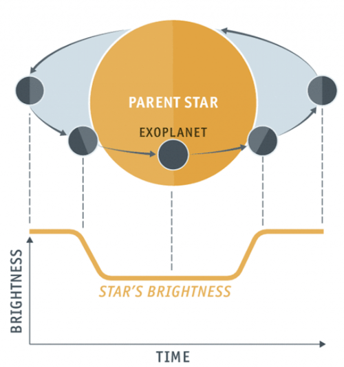
Figure 1. Illustration of the transit of an exoplanet in front of its host star and simultaneous evolution of its brightness with time. The apparent brightness of the star drops when the planet passes between the observer and the star.
Credit: The economist
2Several methods exist to detect exoplanets, yet, one of them is particularly straightforward to explain and very prolific, the so-called transits method. This method works as follow:
3- Given a suitable alignment, the exoplanet can block out a fraction of the starlight causing a small dip in the star’s brightness as seen by the observer (Figure 1). This eclipse of the host star by the planet is called a transit.
4- The amount of missing starlight (depth of the transit) tells us about the size ratio between the transiting planet and its host star. As we can generally measure the size of the star via other methods, we can use the transit depth to infer the size of the planet. More precisely, the depth of the transit is often called dF and is defined by Equation 1:
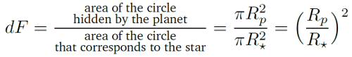
5where Rp is the radius of the planet and R⁎ is the radius of the host star. The larger the depth of the transit the easier it is to detect. Consequently, for a given planet size we will have more chances to detect it around a small star as explained on Figure 2. We will come back to this aspect in the second section of the paper, Section 2.
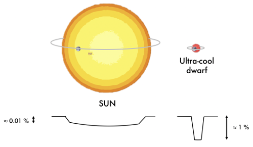
Figure 2. Illustration of the impact of the size of the star of the depth on the transit.
Credit: Elsa Ducrot.
6- This effect repeats itself at every orbital period, P, of the planet (365 days for the Earth around the sun for example). Once we have the period of a planet we can deduce how far it orbits from its star, often referred to as a.
7- However, this method requires that the planet passes exactly between the observer (on Earth) and the host star and this configuration is not very likely. Indeed, the probability of observing a transit for any given star, seen from a random direction and at a random time, is extremely small, as shown on Figure 3. The probability of transit can be approximated to ≈ R⁎/a, where R⁎ is the radius of the star and a the semi-major axis defined above. This means that for an earth-like planet orbiting a sun-like star we would have only ≈0.47% chances to observe one of its transits!
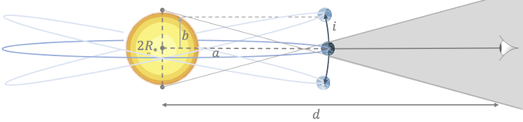
Figure 3. Illustration of the geometry of the transit of an exoplanet in front of its host star. The grey zone show the positions from which the planet will be seen transiting its host star. Out of the grey zone the observer will not be able to see the planet transiting.
Credit: Elsa Ducrot.
8Because a particular alignment is required the transit method can not be used to detect any planet. Fortunately, for the planets that can not be detected via transit other methods exist such as the radial velocity method. Before explaining how this detection method works, we must recall that the first convincing exoplanet detection was made by radial velocity measurements in 1995 [1]. This method is slightly less intuitive than the transit method but it is nevertheless based on physics that we experience every day, namely the Doppler effect. As a reminder, the Doppler effect (or Doppler shift) can be described as the modification of the frequency of a wave emitted by a moving source. There is an apparent upward shift in frequency for observers towards whom the source is approaching and an apparent downward shift in frequency for observers from whom the source is receding. Everyone has already experienced the Doppler effect with sound waves, when a fire-truck passes next to you for instance. Indeed, as the fire-truck approaches with its siren blasting, the sound waves are compressed and the siren sounds higher-pitched, and then suddenly after the truck passes by, the sound waves are stretched and the siren sounds lower-pitched. That is the Doppler effect which can be observed for any type of waves – water waves, sound waves and in our case light waves. Since the light from a star is an electromagnetic wave, like for sound wave, it can be stretched or compressed depending on the motion of the star. Besides, if the planet is gravitationally attracted by its star, the star is also attracted by its planet. Both the planet and the star therefore revolve around a point called the common centre of mass. In the presence of a planet, the star orbits around the centre of mass as it emits light towards us. Similarly to the fire-truck, those electromagnetic waves are compressed when the star moves towards us, such that the star’s light shifts towards the blue in the same way the sound of the pitch of the truck’s siren was getting higher-pitched. Then, those electromagnetic waves are stretched when the star moves away from us and the star’s light shifts to the red. This is shown in Figure 4.
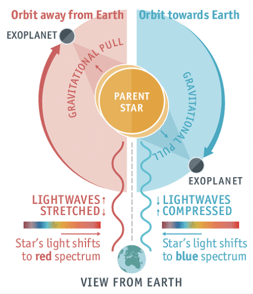
Figure 4. Illustration of the radial velocity method for the detection of exoplanet. The light of the star is shifted towards the blue or the red depending on the motion of the star around the centre of mass of the star-planet system.
Credit: The economist
9This is the basic principle of the radial velocity method. Thanks to the observation of the displacements of known spectral-line in the light emitted by a star, astronomers are able to assess the presence of an exoplanet around this particular star. A remarkable advantage of this method is that it allows to estimate the mass of the planet. However, there is a practical limitation to the sensitivity of the radial-velocity method: stellar activity. As a matter of fact, stars aren’t featureless, they have brighter (hotter, hence bluer) patches called faculae and dimmer (cooler, hence redder) patches called spots. As the star rotates, these patches come in and out of view and these variations in stellar color can look similar to radial-velocity signals from small, close-in planets. Unfortunately, the radial velocity method is not appropriate to the study of planetary system like the TRAPPIST-1 system. Indeed, The faintness of the host star is a limiting factor in the precision, such that the TRAPPIST-1 planets radial velocity signals are beyond the reach of existing instruments. Some spectrographs (instruments used to measure radial velocities) like the Spectro-Polarimetre Infra-Rouge (SPIRou) [2] have started the exploration of habitable Earth-like planets around nearby UCDs stars. Yet simulations, as presented in [3], show that even SPiRou will not be able to provide reliable mass estimates for the TRAPPIST-1 planets.
2. The detection of the TRAPPIST-1 system
10The SPECULOOS project (Search for Planets Eclipsing ULtra-cOOl Stars, [4]) searches for potentially habitable exoplanets around the smallest and coolest stars in our neighbourhood. The stars targeted by SPECULOOS are called ultra-cool dwarfs (UCDs) stars, their effective temperature is lower than 2700 K, their luminosity is lower than 0.1% that of the Sun and their size is closer to the one of Jupiter than the Sun. For several reasons UCDs are ideal targets to search for transiting temperate rocky worlds and characterise their atmosphere:
11• First, their small size leads to deeper transits for Earth-sized planets than what can be obtained for an Earth-Sun twin systems, as seen on Figure 2.
12• UCDs’ habitable zone are also much closer to the host star than for solar-type stars, making the transits of potentially habitable planetsmore likely and more frequent.
13• UCDs are also the most abundant population of star in the solar neighbourhood. There are way more UCDs close to us than sun-like stars.
14SPECULOOS is based on a network of robotic ground-based telescopes that is performing a transit search on the one thousand nearest ultracool dwarf stars [4]. To this date, approximately 200 stars have been monitored during ~100h. SPECULOOS telescopes can be found at three different location on Earth: first, the SPECULOOS South Observatory (SSO) with four 1.0-m telescopes located at the European Paranal Observatory in the Atacama Desert of Chile, then the SPECULOOS Northern Observatory (SNO) with 1 telescope located at Tenerife, Canaries Island, and the SAINT-EX observatory with 1 telescope located at San Pedro de Martir, Mexico. Since 2019 all telescopes are in operation and collecting data [5, 6].
15Yet, the SPECULOOS project actually started a long time ago, in 2011, with its prototype, TRAPPIST, a small robotic telescope located in Chile, monitoring the brightness of a sample of fifty nearby ultracool dwarfs [7]. The purpose of this prototype was to assess the feasibility of the SPECULOOS project, notably in terms of precision and variability of these UCDs. The prototype on TRAPPIST did way more than validating the feasibility of the SPECULOOS project as it provided the first signs ever of the existence of transiting planets around the star 2MASS J23062928-0502285. The first detection of an orbiting object around an UCD star was performed by the TRAPPIST telescope in Sept 2015. TRAPPIST is a 60cm semi-robotic telescope located in La Silla, Chile, a picture is shown on Figure 5 [8]. This UCD star was then renamed TRAPPIST-1 because of the telescope’s name. This announcement was already a major breakthrough as it presented the detection of three Earth-sized planet orbiting a rather close by (40 light-years away), small star (Jupiter-sized) in the Aquarius constellation (at this time only the planet b, c and g as we call them today) [9]. Because of the small size of the host star the signal detection was relatively strong and the period of the planets rather short, which allowed to gather a large number of transits in a small amount of time. But this was only the beginning of the TRAPPIST-1 venture. Indeed, once the TRAPPIST team got several transits on TRAPPIST-1 they asked for follow up time on larger telescopes such as the Very Large Telescope (VLT) located in Paranal, Chile. A night of observation with the VLT revealed a multiple transit, that is to say several planets transiting at the same time. At first sight, the team thought two of the planets they already discovered with TRAPPIST were transiting (planet c and g, as we call them today) but actually additional observations with the Spitzer space based telescope revealed that the event observed with the VLT was a triple transit of one known planet (planet c) with two unknown smaller ones (planet e and f)!
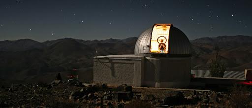
Figure 5. TRAPPIST-South telescope located in La Silla Observatory, Chile.
Credit: Emmanuel Jehin.
Follow-up observations
16Because the three planets discovered represented an exceptional opportunity for the atmospheric characterisation of temperate terrestrial exoplanets with upcoming space telescopes, an intensive follow-up monitoring TRAPPIST-1 was initiated. More than 1000 hours of observations on the space infrared Sptizer telescope (spread over 3 years from February 2016 October to 2019) were granted to look for additional planets and intensively monitor the planets’ transits. This resulted in strong constraints on their masses, sizes, compositions, dynamics, and to explore the system for new transiting planets.
17Those 1500 hours of observation were split in 6 campaigns with the particularity that the second campaign was 20 days of continuous monitoring, which is an extremely unique opportunity. Figure 6 shows the complete set of data acquired by Spitzer, one tiny blue point represents one image from which the flux of the star is measured.
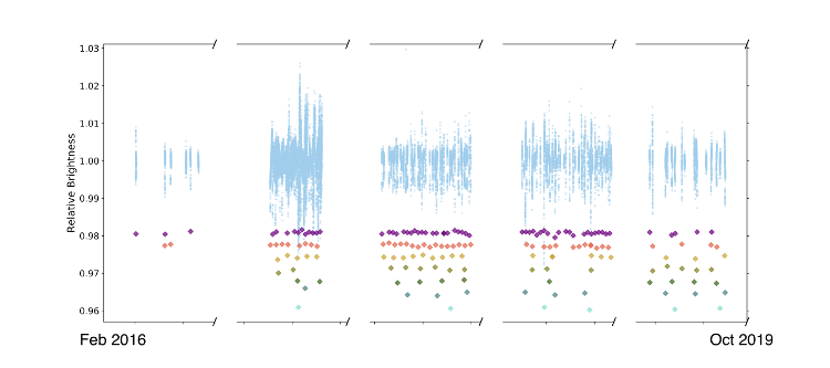
Figure 6. Spitzer photometric measurements (blue) resulting from observations of the star from February 2016 to October 2019 cleaned of data gaps between the four campaigns. Coloured diamonds show the positions of the transits of the different planets with their corresponding depth plus an offset by planet for clarity.
Figure from [10].
18The results from this intensive monitoring from space were tremendous. First and foremost, the follow-up observations revealed 4 additional planets (seven in total) all close to or within the habitable zone of the star [11]. Secondly, those planets are all very well aligned and it is very likely that all of the planets orbit on the same hemisphere of the star [12]. The planets also have very short orbital periods, between 1.5 and 18 days [13] and the system is very compact such that the distance from the planets to the star are ranging from 1% to 6% the distance between the Sun and the Earth. Besides, although the distance between the planets are relatively small (only a few times the Earth-Moon distance) the system appears to be very stable. This stability is due to a peculiar dynamical architecture where the orbital periods of the planets are commensurate, i.e. their values are related by ratios of integer numbers [14], we say that the seven TRAPPIST-1 planets are in mean-motion orbital resonance. Such resonances also occur in the Solar System, with the typical case being the Laplace resonance among Jupiter’s satellites. Specifically, for every time Ganymede orbits Jupiter, Europa orbits twice and Io makes four trips around the planet. This 1:2:4 resonance is considered stable and if one moon were nudged off course, it would selfcorrect and lock back into a stable orbit. In the case of the TRAPPIST-1 system this resonance causes the push of one planet by another to be always nearly compensated by the opposite push from another planet, i.e strong gravitational interactions between the planets but in a way that the sum of their interactions average out. It is this harmonious influence between the seven TRAPPIST-1 siblings that keeps the system stable. Finally, similarly to Jupiter’s moons or to our own moon the tidal influence of TRAPPIST-1 (which is much more massive than its planets) should have trapped the planets in a synchronous rotation state which means their rotation period should equal their orbital period, meaning they always exhibit the same hemisphere to their star.
19Gathering such a large amount of data on one system only was already a great accomplishment and the outcomes were so extraordinary that at the time of shut down of Spitzer in January 2019 the TRAPPIST-1 system was listed as one of its most valuable scientific achievement, all fields considered.
3. Transit timing variations
20The resonant property of the TRAPPIST-1 system that we mentioned before is a unique feature. First, because it led to the discovery of planet h. As a matter of fact, this complex but predictable pattern in the frequency at which each of the six innermost planets orbit their star was unravelled by Spitzer data. The relationships between the planet’s periods suggested that by studying the orbital velocities of its neighbouring planets, the exact orbital velocity of planet h could be predicted, and hence its orbital period. Six possible resonant periods for planet h that would not disrupt the stability of the system were calculated, but only one was not ruled out by existing observations. Indeed, there was a lack of obvious additional transits at the expected times for five of these periods, the only remaining period that could not be ruled out was 18.766 days. Carefully planned follow up observations were able to confirm the presence of planet h. This new discovery of a planet from the study of the motion of other planets in the system is a great example of what happens when theory and observation matches perfectly, and on several aspects it recalls the story of discovery if Neptune.
21Furthermore, in a compact system like TRAPPIST-1, the gravitational pull of the planets among themselves causes one planet to accelerate and another planet to decelerate along its orbit. This implies that the time between transits is not exactly the same over the course of observations. Indeed, the transits of a distant star by a single planet on a Keplerian orbit occur at time intervals exactly equal to the orbital period [15]. However, if an additional planet orbits the same star, the orbits are not Keplerian anymore and the transits are no longer exactly periodic. In this situation, for a given planet we observe the planet’s transit earlier or later than predicted, depending whether it is accelerated by neighbouring planets or decelerated. Those changes in the timing of the transits of a given planet are called transit timing variations or in short TTVs. This effect is explained in Figure 7 which was taken from [15].
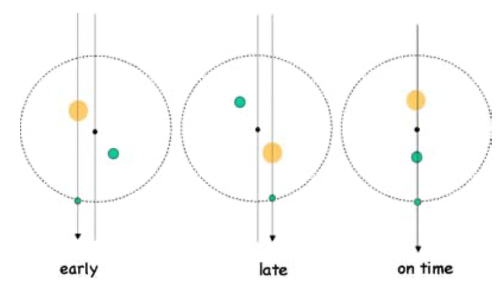
Figure 7. Schematic diagram showing changes in the timing of transit due to a perturbing planet inside the orbit of a transiting planet.
Figure from [15]
22TTVs are further amplified when planets are in mean resonance motion - like in the TRAPPIST-1 system - because it dramatically increases the exchange of torque at each planet conjunction (when the planets are the closest to each other) [16]. In this peculiar situation, some analytical methods exist (refer as TTV inversion problem) to infer the masses of the planets from the monitoring of their transit timings compared to TTV models. This means that the TTVs provide us with an additional method to measure the mass of the planets in an exoplanetary system, without having to rely on radial velocity. Considering the TRAPPIST-1 system is not an appropriate target for radial velocity (as we mentioned before), TTVs are the only solution to get the masses of the planets. The fact that the planets are in resonance is therefore an amazing opportunity for their characterisation.
23In order to get precise masses, we need a large amount of transits for each planet. From those transits, we extract the transit timings (mid-transit times), compute the deviation between the predicted value (if no additional bodies perturbed the orbit of the planet) foreach planet and select the model that fits the observations the best. The best-fit model outputs the masses of all the planets with a precision that depends on the both the quantity and quality of the data (error bars on the transit timings and therefore on the photometry). To this date, we managed to gather 447 transits of all TRAPPIST-1 planets from a combination of ground-based and space-based observations [12]. This includes space-based observations from Kepler, Hubble and Spitzer, and ground-based observations from TRAPPIST, SPECULOOS, the Liverpool telescope, the Very Large Telescope (VLT), United Kingdom Infra-Red Telescope (UKIRT), the Anglo-Australian Telescope (AAT), the Himalayan Chandra Telescope (HCT), and the William Herschel Telescope (WHT).
24Such an extensive data set opens the way towards an in-depth characterisation of the system. A recent publication made use of all available transit timings to analyse the TTVs and refine the masses of the planets [12]. In parallel, another study refined the sizes and ephemeris of the planets [13]. Combining these two measurements, densities of the seven planets were derived. The resulting values revealed that the planets’ densities range from 75% to 99% the density of the Earth [12].
25Being able to derive the densities of the planets while solely relying on transit information is a key asset of the TRAPPIST-1 system and it enables to question the planets interiors. Indeed, although we can not examine the interiors of planets directly (not even our own Earth), we can still construct models that compute what are the most likely interior compositions and fit them to existing data. Figure 8 shows were the TRAPPIST-1 planets stand in terms of mass and radius and how compatible it is with different scenarios from the planets’ interior composition.
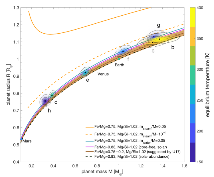
Figure 8. Mass-radius relation for the seven TRAPPIST-1 planets based on the transit-timing and photodynamic analysis from [12].
Each planet is coloured by the equilibrium temperature with the intensity proportional to probability. The solid blue line was calculated for a 5% water composition and 75% of Fe/Mg, for irradiation low enough (i.e. for planets e, f, g and h) that water is condensed on the surface (assuming a surface pressure of 1 bar and a surface temperature of 300 K). The orange dashed and solid lines were calculated for a 0.01% and a 5% water composition, respectively and 75% of Fe/Mg, for irradiation high enough (i.e. for planets b, c and d) that water has fully evaporated in the atmosphere. The Earth (i.e 83% of Fe/Mg), Venus and Mars are plotted as single points, also coloured by their equilibrium temperatures. Figure from [12]
26Figure 8 was taken from [12] and it reveals that the TRAPPIST-1 planets may all have an Earth-like iron/rock composition, but then also require an additional volatile enhancement, such as an outer water layer or a core-free structure with oxidised iron in the mantle.
27These compositions and the unique dynamical structure of the system seem to favour a scenario where the planets formed much further away from the star, in the outer, water-rich part of the protoplanetary disk, and only later migrated closer to the star because of interactions with the gaseous part of the disk.
4. Transit transmission spectra
28In the previous paragraph we presented how we can constrain the interiors of planets from transits only. In this section we show another amazing advantage of the transit method but this time to probe the atmosphere (if any) of the planets.
29As the light emitted by the star passes through a planet atmosphere, it interacts with the molecules and particles present. In the atmosphere, electromagnetic radiation (i.e light from the star) can be scattered, reflected or absorbed. The transmissivity of the atmosphere is defined as the percentage of light that gets through by the atmosphere. A transmissivity of 0.5 means that only 50% of the light passes through the atmosphere. This quantity depends on many parameters including the wavelength of the incoming radiation, the thickness and composition of the atmosphere, etc. For example on earth visible light and radio waves can pass relatively freely through the atmosphere, while X-Rays cannot.
30In parallel, in laboratories, the transmission spectra of each known molecules have been extensively studied. Every one of them has its own spectral signature. For instance, we know that CO2 primarily absorbs radiation in the mid and far (thermal) infrared and that H2O has absorption bands in the mid-infrared and the near-infrared.
31This knowledge allows astrophysicists to probe exoplanets’ atmosphere as illustrated in Figure 9. We use the fact that at certain wavelengths molecules of the planet’s atmosphere absorb light (in the blue band on the figure) whereas at other wavelengths it does not (in the red bands). As a result, from the observer point of view, less light will be absorbed in the blue that in the red, meaning that the planet looks larger in the blue than in the red. Consequently, the transit will be deeper in the blue band than in the red band. Those variations in transit depth due to the atmosphere are very small compared to the depth of the transit itself. This method for atmospheric characterisation of exoplanets is called transit transmission spectroscopy. From the transit transmission spectra of exoplanets we can identify known molecular signatures and unravel the atmospheric composition. The best candidates for transmission spectroscopy studies are transiting planets with a relatively large size compared to their host star in order to increase the significance of transit depth variations due to the planets atmosphere. Furthermore, short period planets are favoured because it is easier to get transits and fold them. This explains why, to date, the TRAPPIST-1 system stands among the most exciting candidate for in-depth studies on habitability [17].
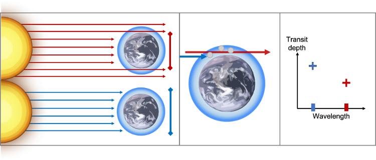
Figure 9. Illustration of the transit transmission spectroscopy technique.
On the left-panel we show that depending on the colour of the light (wavelengths) the radiation are either absorbed or transmitted. On the middle-panel we see that this phenomenon is due to the presence of molecules in the atmosphere that block light at certain wavelengths. On the right-panel we see how this effect translates in terms of transit depth for an observer recording the transit of a planet with an atmosphere in front of its star. Credit: Elsa Ducrot.
32The 447 transits observed with the many telescopes mentioned earlier, were observed in different wavelengths such that transit transmission spectra of the TRAPPIST-1 planets can be constructed [13]. Figure 10 shows the transit transmission spectra of planets b, c, e and g compared with several atmospheric models. We chose to only show those four because planets b and c are the closest (so the one for which we have the most transits), planet e is arguably the most promising candidate for habitability, and planet g was the most observed planet with the Hubble space telescope (from which observations are particularly valuable in terms of transmission spectrum).
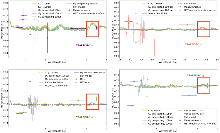
Figure 10. Top-left: Transit transmission spectrum of TRAPPIST-1b from observations compared with simulated transmission spectra derived by [18] for different terrestrial atmospheres. Each colour is associated with a different scenario: - gold stands for 10 or 100 bars CO2-rich atmospheres - salmon stands for 10 or 100 bars O2-rich desiccated atmospheres - green stands for 10 or 100 bars O2-rich outgazing atmospheres - brown stands for 10 or 92 bars Venus-like atmospheres - and blue stands for an aqua planet with either clear or cloudy sky. Red rectangles highlight the presence of a CO2 feature at this wavelength range. Top-right: Similarly for TRAPPIST-1c. Bottom-left: Similarly for TRAPPIST-1e. Bottom-right: Similarly for TRAPPIST-1g.
Figure from [10].
33For the transmission spectrum to be as indicative as possible on the atmospheric composition we need a high resolution (that is to say as many measurements at different wavelengths as possible) and the best precision possible. To this extent, the most appropriate facilities seem to be space based-telescopes equipped with an instrument capable to decompose the electromagnetic radiations in different wavelengths and analyse them one by one (this instrument is called a spectrograph). For this purpose the best instrument at our disposal is currently the Hubble space telescope (HST). One of its instrument called the Wide Field Camera 3 is particularly suited to find indirect evidence of clouds in exoplanets atmospheres because its wavelength range covers one of the hydrogen and water absorption bands.
34Nevertheless, the lack of prominent absorption features in the HST observations rules out cloud-free (and haze-free) hydrogen-dominated atmospheres. This represents a strong constrain because an atmosphere that would be rich in H2 would probably not be a suitable candidate to look for biosignatures. Indeed, although some researches on the possibility of life in these environments are arising [19] we know that a lack of hydrogen probably means that these atmospheres are shallow and rich in heavier gases like those found in the Earth’s atmosphere, such as carbon dioxide, methane and oxygen. Furthermore, based on the masses and radii measurements [12, 13, 16], the TRAPPIST-1 planets are not compatible with a bare rock composition, meaning that, we would still expect them to have an atmosphere, although not hydrogen-rich. However, if we further compare the existing data points to a series of simulated mean molecular weight (not hydrogen rich) atmospheres, as done on Figure 10, we observe that the precision on our current observation is not good enough to exclude/favour any scenarios. Even the CO2 feature -in red in Figure 10 and the largest feature in those simulated spectra - cannot be confirmed or rejected based on current measurements. Hopefully, these limitations should be overcome with the next generation of telescope, notably the James Webb Space Telescope (JWST) and the Extremely Large Telescope (ELT). We will discuss these future projects in Section 6.
35One important aspect to take into account for intransit transmission spectroscopy is stellar contamination. As we mentioned when we introduced the radial velocity method, the surface of a star is never fully homogeneous. Its photosphere (star’s outer shell from which light is radiated) is covered with a certain percentage of dark spots and bright faculae. Unfortunately, those spots and facalue have a direct impact on the depth of the transits if a planet passes in front of them. In this case, either more light is masked (when the planet hides a bright faculae) or less light is masked (when the planet hides a dark spot). This results in an additional bump or drop of brightness during the transit. This scenario is illustrated on the left-panel of Figure 11 showing a spot-crossing event.
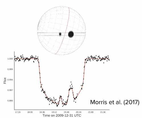
Figure 11. Modelling of the impact of photospheric heterogeneities on one transit of the planet HAT-P-11 b. Occultations of spots by the planet results in an increase of flux during the transit.
Figure from [20], credit: Brett Morris.
36Another example happens when there are unocculted spot/faculae on the star. Unocculted spots/faculae are one manifestation of a generic issue with transit observations called the transit light source effect [21]. Transit transmission spectroscopy consists in comparing the incident light from the disk-integrated stellar spectrum before and during the transit. This is based on the assumption that the disk-integrated spectrum is identical to the light incident on the planetary atmosphere, which is not always the case. Indeed, the planet is not occulting the entire stellar disk but only a small region within the transit chord. Therefore, the light source for the transmission measurement is a small time-varying annulus within the stellar disk defined by the planet’s projection (see Figure 12), the spectrum of which may differ significantly from the disk-averaged spectrum in the presence of spots or faculae on the star. This scenario is illustrated on figure 12.
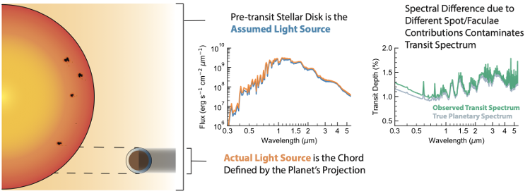
Figure 12. A Schematic of the Transit Light Source Effect. During a transit, exoplanet atmospheres are illuminated by the portion of a stellar photosphere immediately behind the exoplanet from the point of view of the observed. Changes in transit depth must be measured relative to the spectrum of this light source. However, the light source is generally assumed to be the disk-integrated spectrum of the star. Any differences between the assumed and actual light sources will lead to apparent variations in transit depth.
Figure from [21], credit: Benjamin Rackham.
37The direct impact of the transit light source (TLS) effect is that the heterogeneity of the star’s photosphere can mimic the spectral features we would expect from an atmosphere [21], see Figure 13.
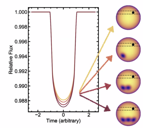
Figure 13. Illustration of the effect of unocculted stellar spot on the depth of the transit of a planet orbiting a spotted star.
Credit: Benjamin Rackham.
38Therefore, understanding and correcting the effects of stellar heterogeneity appears essential to prepare the exploration of TRAPPIST-1’s planets [22]. Several studies [5, 13, 22, 23] do not seem to report any clear spot/faculae-crossing events on TRAPPIST-1 planets’ transits but this does not mean those spot/faculae are not there, as they can also be unocculted. To detect unoculted spots/faculae the only way is to model the TLS effect and look for its spectral signatures in the transmission spectra of the planets. Models are currently being developed to simulate the TLS effect [21, 24]. In the mean time, follow up observations should continue as they help discarding unrealistic estimations of spot/faculae covering fractions.
5. Habitability
39One of the most important question concerning the TRAPPIST-1 planets is their potential habitability. We stated in the introduction of this article that three out of the seven planets (planets e, f and g) are in the habitable zone of TRAPPIST-1, meaning these planets could have liquid water on their surface and therefore have the preconditions for life as we know it on Earth. Nevertheless, many additional aspects need to be properly accounted for before we can confirm/reject the presence of life on one of these planets. In the previous section we discussed the transmission spectroscopy and the impact of stellar contamination on its interpretation. It turns out that the star’s activity also plays a role in the emergence of life.
40Some stars can undergo unpredictable short dramatic increases in brightness called flares associated to important release of UV energy, they show a very specific pattern in a light-curve (sudden increase followed by an exponential decay, see Figure 14).
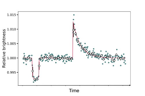
Figure 14. Example of a flare captured after a transit of TRAPPIST-1b observed with the Spitzer space telescope.
Figure from [10].
41However, flares may erode exoplanets’ atmospheres and impact their habitability. UCDs like TRAPPIST-1 are likely to exhibit flares, as confirmed by several publications [13, 25, 26]. Furthermore, as the planets are very close to the star, they are much more irradiated than the Earth. In this context, the study of flares is essential to gain insights on planetary evolution and the potential presence of life. On one hand, intense flare activity can induce strong atmospheric erosion and make the surface of a planet uninhabitable [27], but on the other hand flares could be a key element to the emergence of life [28, 29]. Indeed, some laboratory experiences show that a minimum flaring activity seems beneficial to the formation of pyrimidine, the ribonucleotide that will allow ribonucleic acid (RNA) synthesis and initiate prebiotic chemistry [30].
42From this discovery, the authors of this study defined the “abiogenesis zones”, a zone around stars that depends on whether UV fluxes provide sufficient energy to build a sufficiently large prebiotic inventory [30]. For a planet orbiting a UCD to be in the abiogenesis zone, it needs to receive a minimum amount of UV flux which translates in constraints on the minimum flare frequency and minimum energy for those flares.
43In the extensive data set that we have at our disposal, several flares were identified and their energies and frequency were derived [13, 25, 26]. Comparing these results with calculations from [30] it was found that the TRAPPIST-1 habitable zone planets currently do not receive enough UV flux to build up the prebiotic inventory photochemically. Yet, TRAPPIST-1 is a rather old star (7.6±2.2 Gyr old according to [31]) and empirical observations predict a decrease of the activity of UCD stars over time, meaning TRAPPIST-1 might have exhibited more energetic and more frequent flares in its youth. In this case, the planets that lie within the habitable zone today might have also reside in the abiogenesis zone some time ago. Last but not least, contrary to the habitable zone, it is not required that a planet remains in the abiogenesis zone of its star to maintain the presence of life. This would imply that some of the TRAPPIST-1 habitable zone planets might have received enough UV flux in their history to drive the emergence of life’s building blocks.
6. Future prospects
44As we already mentioned several times in this article the TRAPPIST-1 planets are well-suited for a detailed atmospheric characterization with the upcoming James Webb Space Telescope (JWST). JWST is a 6m-aperture infrared space telescope, the largest telescope ever sent in space, and it will be able to probe the planets’ atmospheric compositions, constrain their surface properties and assess their habitability. It could even detect molecules of possible biological origins [18, 32–34]. Its launch is now scheduled for 2021. Several simulations of the capabilities of JWST observations for TRAPPIST-1 planets show very promising results. For instance, molecular absorption features may be detectable with JWST in ~2-15 transits. In particular we are pretty convinced that we should be able detect CO2 features in transit transmission spectrum of planet b with less then 5 transits as shown by Figure 15.
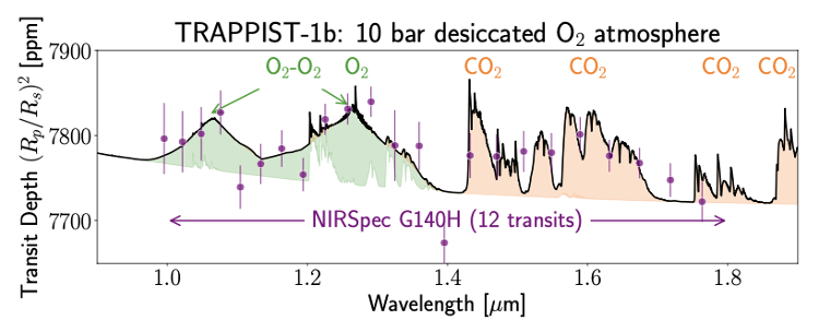
Figure 15. Theoretical transmission spectra of TRAPPIST-1 b assuming a 10 bar desiccated O2 atmosphere atmospheric compositions (in solid black line) compared to modelled measurements with error bars calculated for 12 transits observed with JWST NIRSpec G140H (purple dots).
Figure from [33].
45Besides, giant ground based telescopes such as the Extremely Large Telescope (ELT) should also be able to shed some light on the atmospheric composition of the TRAPPIST-1 planets atmospheres. Specifically, detection of molecules such as H2O or O2 could be attempted on the ELT [35], although the number of required transits may be prohibitively large, especially if clouds turn out to be present in the atmospheres.
46Finally, a series of proposed future observatories intent to observe the TRAPPIST-1 system with some of them predicting remarkable results, like the Origins [36] or LUVOIR [37] space telescopes. Figure 16 shows the gain from JWST to Origins for the observation of 60 transits of TRAPPIST-1e. We see that the Origins space telescope would provide us with measurements precise enough to detect O3 in the atmosphere of planet e, which could be an important signature for confirming the presence of life (a biosignature).
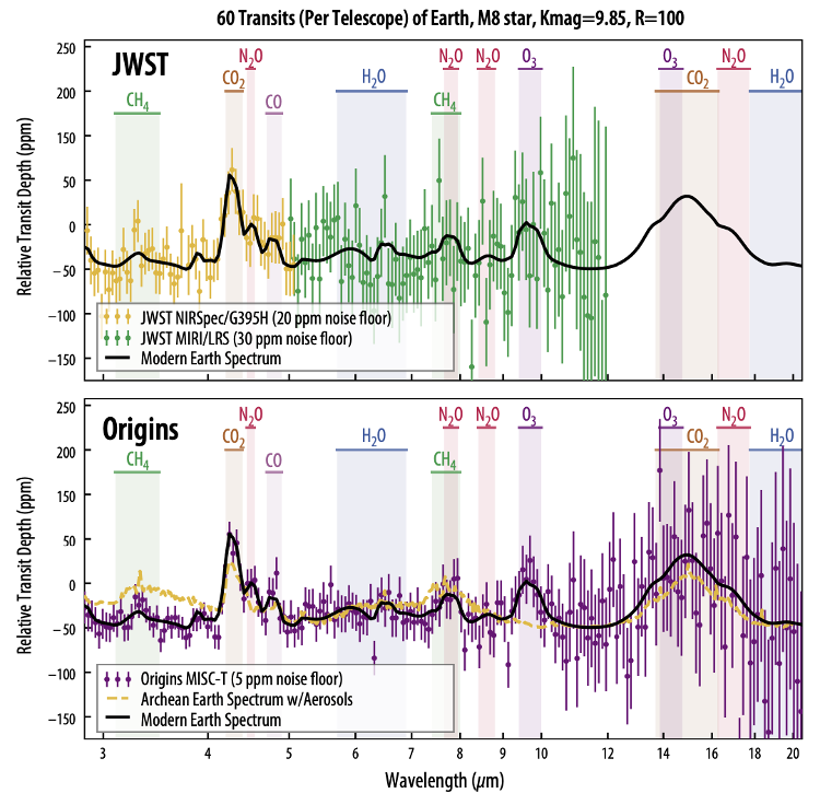
Figure 16. Simulated transmission spectra for a TRAPPIST-1e-like planet with an Earth-like composition (60 transits), comparing JWST and Origins measurements based on current best estimates for their respective instrument noise
(20 – 30 ppm for JWST; 5 ppm for Origins)
47Yet, there is still a long way to go from biosignatures to life as many false positive and false negative exists, like O2. Indeed, one could think dioxygen is the perfect biosignature but it could very well be possible to find O2 in the atmosphere of a planet with no life on, or viceversa (such as the Earth at the time of the Archean).
48In this article we reviewed the history of the discovery of the TRAPPIST-1 system and explained why it is an exceptional target for in-depth characterisation. Since its discovery, only four years ago, more than 500 papers are already mentioning TRAPPIST-1 according to the astrophysics data system ADS. A lot of efforts are still needed to unravel the secrets of the planets and the impact of their star but we believe the exploration of TRAPPIST-1 system could entirely change our paradigm and pave the way towards a better understanding of the evolution of the atmospheres and habitability of terrestrial planets.
7. Learn more about SPECULOOS and TRAPPIST-1
49If you are interested in learning more about the SPECULOOS project, the amazing TRAPPIST-1 system and exoplanets in general, here are some links to websites and videos you might find useful to guide your research:
50• Introduction to exoplanets (in french):
51https://www.explore-exoplanets.eu/playlist/exoplanetes-recherche-spatiale/
52• Introduction to exoplanets (in english):
53https://www.youtube.com/watch?v=Ppc1N3k8pYY&ab_channel=SpaceTelescopeScienceInstitute
54• Introduction to Astrobiology (in french):
55https://www.youtube.com/watch?v=qcs8cZHVQ2c&ab_channel=Europlanet
56• Introduction to Astrobiology (in english):
57https://www.youtube.com/watch?v=SOzZnVxIgsc&ab_channel=Europlanet
58• SPECULOOS project:
59https://www.speculoos.uliege.be/cms/c_4259452/en/speculoos
60• Presentation of SNO:
61https://www.youtube.com/watch?v=jEUpbGgu-D4&ab_channel=Earth%2CAtmosphericandPlanetarySciencesMIT
62• Presentation of SSO:
63https://www.youtube.com/watch?v=YqwSnCxFoDo&ab_channel=Universit%C3%A9deLi%C3%A8ge
64• Personal website of the TRAPPIST-1 system:
66• TRAPPIST-1 resonant chain in images and sound:
67https://www.youtube.com/watch?v=WS5UxLHbUKc&ab_channel=SYSTEMSounds
68• The university of Liège’s summary of the first year following the discovery of the TRAPPIST-1 system:
Bibliographie
[1] M. Mayor, D. Queloz, Nature 1995, 378, Number:6555 Publisher: Nature Publishing Group, 355–359.
[2] J. F. Donati, D. Kouach, M. Lacombe, S.Baratchart, R. Doyon, X. Delfosse, E. Artigau, C. Moutou, G. Hebrard, F. Bouchy, J. Bouvier, S. Alencar, L. Saddlemyer, L. Pares, P. Rabou, Y. Micheau, F. Dolon, G. Barrick, O. Hernandez, S. Y. Wang, V. Reshetov, N. Striebig, Z. Challita, A. Carmona, S. Tibault, E. Martioli, P. Figueira, I. Boisse, F. Pepe, arXiv:1803.08745 [astro-ph] 2018, arXiv: 1803.08745, 903–929.
[3] B. Klein, J.-F. Donati, Monthly Notices of the Royal Astronomical Society 2019, 488, arXiv: 1907.05710, 5114–5126.
[4] L. Delrez, M. Gillon, D. Queloz, B.-O. Demory, Y. Almleaky, J. de Wit, E. Jehin, A. H. M. J. Triaud, K. Barkaoui, A. Burdanov, A. J. Burgasser, E. Ducrot, J. McCormac, C. Murray, C. S. Fernandes, S. Sohy, S. J. Thompson, V. Van Grootel, R. Alonso, Z. Benkhaldoun, R. Rebolo, arXiv:1806.11205 [astro-ph] 2018, arXiv: 1806.11205.
[5] L. Delrez, M. Gillon, A. H. M. J. Triaud, B.-O. Demory, J. deWit, J. G. Ingalls, E. Agol, E. Bolmont, A. Burdanov, A. J. Burgasser, S. J. Carey, E. Jehin, J. Leconte, S. Lederer, D. Queloz, F. Selsis, V. Van Grootel, Monthly Notices of the Royal Astronomical Society 2018, 475, arXiv: 1801.02554, 3577–3597.
[6] D. Sebastian, M. Gillon, E. Ducrot, F. J. Pozuelos, L. J. Garcia, M. N. Günther, L. Delrez, D. Queloz, B. O. Demory, A. H. M. J. Triaud, A. Burgasser, J. de Wit, A. Burdanov, G. Dransfield, E. Jehin, J. McCormac, C. A. Murray, P. Niraula, P. P. Pedersen, B. V. Rackham, S. Sohy, S. Thompson, V. Van Grootel, arXiv:2011.02069 [astro-ph] 2020, arXiv: 2011.02069.
[7] M. Gillon, A. H. M. J. Triaud, J. J. Fortney, B.-O. Demory, E. Jehin, M. Lendl, P. Magain, P. Kabath, D. Queloz, R. Alonso, D. R. Anderson, A. Collier Cameron, A. Fumel, L. Hebb, C. Hellier, A. Lanotte, P. F. L. Maxted, N. Mowlavi, B. Smalley, Astronomy & Astrophysics 2012, 542, A4.
[8] E. Jehin, M. Gillon, D. Queloz, P. Magain, J. Manfroid, V. Chantry, M. Lendl, D. Hutsemékers, S. Udry, The Messenger 2011, 145, 2–6.
[9] M. Gillon, E. Jehin, S. M. Lederer, L. Delrez, J. de Wit, A. Burdanov, V. Van Grootel, A. J. Burgasser, A. H. M. J. Triaud, C. Opitom, B.-O. Demory, D. K. Sahu, D. Bardalez Gagliuffi, P. Magain, D. Queloz, 2016, 533, 221–224.
[10] E. Ducrot, M. Gillon, L. Delrez, E. Agol, P. Rimmer, M. Turbet, M. N. Günther, B.-O. Demory, A. H. M. J. Triaud, E. Bolmont, A. Burgasser, S. J. Carey, J. G. Ingalls, E. Jehin, J. Leconte, S. M. Lederer, D. Queloz, S. N. Raymond, F. Selsis, V. Van Grootel, J. de Wit, Astronomy & Astrophysics 2020, arXiv: 2006.13826, DOI 10.1051/0004-6361/201937392.
[11] M. Gillon, A. H. M. J. Triaud, B.-O. Demory, E. Jehin, E. Agol, K. M. Deck, S. M. Lederer, J. de Wit, A. Burdanov, J. G. Ingalls, E. Bolmont, J. Leconte, S. N. Raymond, F. Selsis, M. Turbet, K. Barkaoui, A. Burgasser, M. R. Burleigh, S. J. Carey, A. Chaushev, C. M. Copperwheat, L. Delrez, C. S. Fernandes, D. L. Holdsworth, E. J. Kotze, V. Van Grootel, Y. Almleaky, Z. Benkhaldoun, P. Magain, D. Queloz, Nature 2017, 542, 456–460.
[12] E. Agol, C. Dorn, S. L. Grimm, M. Turbet, E. Ducrot, L. Delrez, M. Gillon, B.-O. Demory, A. Burdanov, K. Barkaoui, Z. Benkhaldoun, E. Bolmont, A. Burgasser, S. Carey, J. de Wit, D. Fabrycky, D. Foreman-Mackey, J. Haldemann, D. M. Hernandez, J. Ingalls, E. Jehin, Z. Langford, J. Leconte, S. M. Lederer, R. Luger, R. Malhotra, V. S. Meadows, B. M. Morris, F. J. Pozuelos, D. Queloz, S. M. Raymond, F. Selsis, M. Sestovic, A. H. M. J. Triaud, V. Van Grootel, arXiv:2010.01074 [astro-ph] 2020, arXiv:2010.01074.
[13] E. Ducrot, M. Gillon, L. Delrez, E. Agol, P. Rimmer, M. Turbet, M. N. Günther, B.-O. Demory, A. H. M. J. Triaud, E. Bolmont, A. Burgasser, S. J. Carey, J. G. Ingalls, E. Jehin, J. Leconte, S. M. Lederer, D. Queloz, S. N. Raymond, F. Selsis, V. Van Grootel, J. de Wit, Astronomy & Astrophysics 2020, 640, A112.
[14] R. Luger, J. Lustig-Yaeger, E. Agol, The Astrophysical Journal 2017, 851, arXiv: 1711.05739, 94.
[15] E. Agol, J. Steffen, R. Sari, W. Clarkson, Monthly Notices of the Royal Astronomical Society 2005, 359, 567–579.
[16] S. L. Grimm, B.-O. Demory, M. Gillon, C. Dorn, E. Agol, A. Burdanov, L. Delrez, M. Sestovic, A. H. M. J. Triaud, M. Turbet, Bolmont, A. Caldas, J. de Wit, E. Jehin, J. Leconte, S. N. Raymond, V. Van Grootel, A. J. Burgasser, S. Carey, D. Fabrycky, K. Heng, D. M. Hernandez, J. G. Ingalls, S. Lederer, F. Selsis, D. Queloz, Astronomy & Astrophysics 2018, 613, arXiv: 1802.01377, A68.
[17] M. Turbet, E. Bolmont, V. Bourrier, B.-O. Demory, J. Leconte, J. Owen, E. T. Wolf, arXiv:2007.03334 [astro-ph physics:physics] 2020, arXiv: 2007.03334.
[18] A. P. Lincowski, V. S. Meadows, D. Crisp, T. D. Robinson, R. Luger, J. Lustig-Yaeger, G. N. Arney, The Astrophysical Journal 2018, 867, arXiv: 1809.07498, 76.
[19] S. Seager, J. Huang, J. J. Petkowski, M. Pajusalu, Nature Astronomy 2020, 4, 802–806.
[20] B. M. Morris, L. Hebb, J. R. A. Davenport, G. Rohn, S. L. Hawley, 2017, 846, 99.
[21] B. V. Rackham, D. Apai, M. S. Giampapa, The Astrophysical Journal 2018, 853, arXiv: 1711.05691, 122.
[22] E. Ducrot, M. Sestovic, B. M. Morris, M. Gillon, A. H. M. J. Triaud, J. de Wit, D. Thimmarayappa, E. Agol, Y. Almleaky, A. Burdanov, A. J. Burgasser, L. Delrez, B.-O. Demory, E. Jehin, J. Leconte, J. McCormac, C. Murray, D. Queloz, F. Selsis, S. Thompson, V. Van Grootel, The Astronomical Journal 2018, 156, arXiv: 1807.01402, 218.
[23] B. M. Morris, E. Agol, L. Hebb, S. L. Hawley, M. Gillon, E. Ducrot, L. Delrez, J. Ingalls, B.-O. Demory, The Astrophysical Journal 2018, 863, arXiv: 1808.02808, L32.
[24] S. E. Moran, S. M. Hörst, N. E. Batalha, N. K. Lewis, H. R.Wakeford, The Astronomical Journal 2018, 156, 252.
[25] K. Vida, Z. Kovári, A. Pál, K. Oláh, L. Kriskovics, The Astrophysical Journal 2017, 841, arXiv: 1703.10130, 124.
[26] J. R. A. Davenport, K. R. Covey, R. W. Clarke, A. C. Boeck, J. Cornet, S. L. Hawley, The Astrophysical Journal 2019, 871, arXiv: 1901.00890, 241.
[27] H. Lammer, H. I. Lichtenegger, Y. N. Kulikov, J.-M. Grießmeier, N. Terada, N. V. Erkaev, H. K. Biernat, M. L. Khodachenko, I. Ribas, T. Penz, F. Selsis, Astrobiology 2007, 7, 185–207.
[28] V. S. Airapetian, A. Glocer, G. Gronoff, E. Hébrard, W. Danchi, Nature Geoscience 2016, 9, 452–455.
[29] S. Ranjan, R. Wordsworth, D. D. Sasselov, 2017, 843, 110.
[30] P. B. Rimmer, J. Xu, S. J. Thompson, E. Gillen, J. D. Sutherland, D. Queloz, Science Advances 2018, 4, eaar3302.
[31] A. J. Burgasser, E. E. Mamajek, The Astrophysical Journal 2017, 845, 110.
[32] C. V. Morley, L. Kreidberg, Z. Rustamkulov, T. Robinson, J. J. Fortney, The Astrophysical Journal 2017, 850, arXiv: 1708.04239, 121.
[33] J. Lustig-Yaeger, V. S. Meadows, A. P. Lincowski, The Astronomical Journal 2019, 158, arXiv: 1905.07070, 27.
[34] T. J. Fauchez, M. Turbet, G. L. Villanueva, E. T. Wolf, G. Arney, R. K. Kopparapu, A. Lincowski, A. Mandell, J. de Wit, D. Pidhorodetska, S. D. Domagal-Goldman, K. B. Stevenson, The Astrophysical Journal 2019, 887, arXiv: 1911.08596, 194.
[35] I. A. G. Snellen, R. J. de Kok, R. le Poole, M. Brogi, J. Birkby, The Astrophysical Journal 2013, 764, 182.
[36] M. Meixner, A. Cooray, D. Leisawitz, J. Staguhn, L. Armus, C. Battersby, J. Bauer, E. Bergin, C. M. Bradford, K. Ennico-Smith, J. Fortney, T. Kataria, G. Melnick, S. Milam, D. Narayanan, D. Padgett, K. Pontoppidan, A. Pope, T. Roellig, K. Sandstrom, K. Stevenson, K. Su, J. Vieira, E. Wright, J. Zmuidzinas, K. Sheth, D. Benford, E. E. Mamajek, S. Neff, E. D. Beck, M. Gerin, F. Helmich, I. Sakon, D. Scott, R. Vavrek, M.Wiedner, S. Carey, D. Burgarella, S. H. Moseley, E. Amatucci, R. C. Carter, M. DiPirro, C.Wu, B. Beaman, P. Beltran, J. Bolognese, D. Bradley, J. Corsetti, T. D’Asto, K. Denis, C. Derkacz, C. P. Earle, L. G. Fantano, D. Folta, B. Gavares, J. Generie, L. Hilliard, J. M. Howard, A. Jamil, T. Jamison, C. Lynch, G. Martins, S. Petro, D. Ramspacher, A. Rao, C. Sandin, E. Stoneking, S. Tompkins, C. Webster, Origins Space Telescope Mission Concept Study Report, 2019.
[37] T. L. Team, The LUVOIR Mission Concept Study Final Report, 2019.
