Mark J. DEKKERS

Magnetic susceptibility as a proxy parameter: assets and pitfalls
André Dumont medalist lecture 2024

Documento adjunto(s)

Anexidades

• GB 29-1-2 Dekkers MJ (3,5M)

Abstract

The merit of the low-field magnetic susceptibility as proxy parameter is concisely reviewed. In many geological samples it is a composite consisting of a diamagnetic, paramagnetic, and ferromagnetic (sensu lato) contribution that varies with rock type. For weakly magnetic samples, the diamagnetic and paramagnetic contributions are an appreciable portion of the measured susceptibility. In such materials equating the measured susceptibility with the ferromagnetic susceptibility is not warranted. Before a susceptibility record is geologically interpreted, the underlying drivers of its variation must be understood. This is achieved by integrating susceptibility data with an extended magnetic property analysis, geochemical information, and a paleomagnetic assessment of the timing of the acquisition of the natural remanent magnetization as the magnetic minerals may post-date the sedimentation age. Measuring the susceptibility at several frequencies and in varying low applied fields provides important information on the grain-size distribution in the ultrafine grain end and, to a lesser extent, on the magnetic mineralogy. Examples discussed include research into loess/paleosol records and high-resolution time scale development. Variable surficial oxidation of magnetite particles and potential remagnetization complicate the interpretation of a susceptibility record in terms of paleoclimate.

Tabla de contenidos

1. Introduction

1The low-field magnetic susceptibility, also referred to as susceptibility here, is widely used as a proxy parameter primarily in paleoclimate reconstructions, high-resolution correlation of coeval sedimentary sequences within a single basin, and the construction of high-resolution time scales, also in deep time. Paleoclimate reconstructions, for example, include its use as a paleorainfall index: higher rainfall, i.e. wetter climate, results in increased soil development and higher run-off from the continent promoting increased deposition of clastic material. Stratigraphic susceptibility records of sufficient resolution are subjected to spectral analysis to search for orbital frequencies. If these can be demonstrated, a high-resolution duration chronometer becomes available which enables to put tight constraints on the rate of paleoenvironmental changes in deep time, difficult to achieve with other methods. Advantages of the susceptibility as a proxy include quick and sensitive measurement, possibility to perform measurements on-site in the field, and its non-destructive nature, so that the same sample can be used afterwards for other determinations. The interpretation of a susceptibility record, however, is often not as unique as one would like, an underappreciated caveat. Susceptibility is a bulk parameter of a rock sample, a reflection of the minerals making up the sample and its geological history. For a sound interpretation these must be understood. In this contribution the basics of susceptibility, its measurement, and how to achieve a less unique interpretation of a susceptibility record are reviewed before showing examples of successful applications in geosciences. We focus on bulk susceptibility and not on the anisotropy of magnetic susceptibility (AMS). Books and informative review papers on AMS include Rochette et al. (1992), Tarling & Hrouda (1993), Borradaile & Henry (1997), Cifelli et al. (2004), and Parés (2015).

1.1. Basic definitions

2The magnetic susceptibility is the magnetic moment M of a substance acquired in a given magnetic field divided by that field (e.g. Dunlop & Özdemir, 1997; Dearing, 1999; Roberts, 2026). It is a material property which can be temperature- and/or field-dependent. The field is typically expressed in units of H (A/m).

3Susceptibility = M/H with dimensions [Am²]/[A m^-1] (1)

4One can express susceptibility on a mass-specific, molar-specific, or a volume-specific basis. Then dimensions of expression (1) are respectively:

5Mass-specific: [Am² kg^-1] / [A m^-1] = [m³ kg^-1] SI symbol: χ

6Molar-specific: [Am² mol^-1] / [A m^-1] = [m³ mol^-1] SI symbol: χ_m

7Volume-specific: [A m^-1] / [A m^-1] = dimensionless number SI symbol: κ

8Implicitly with ‘magnetic susceptibility’ or ‘susceptibility’, one often refers to the low-field or initial susceptibility, measured in field strengths up to ~10–20 times the strength of Earth’s magnetic field, i.e., up to 500–1000 μT (equivalent to ~400–800 A/m). In many geological oriented papers magnetic susceptibility is shortened to MS without being specific whether mass or volume specific susceptibility is implied. Rather often volume-specific susceptibility is implicitly inferred.

9A proper interpretation of a susceptibility proxy record—the variations in susceptibility—may come with challenges and requires a good understanding of the driver(s) of the susceptibility variations. The measured susceptibility K_m of a sample is the sum of the susceptibility of all grains in that sample. Geological samples consist typically of a variety of minerals that each have their specific magnetic properties and may have widely varying susceptibility.

10Magnetic behavior is categorized in several classes. We distinguish diamagnetism, paramagnetism, and ferromagnetism sensu lato. Materials that belong to the first two classes cannot carry a permanent or remanent magnetic moment, colloquially: they are not magnetic. Materials belonging to the third class possess a remanent magnetic moment that can be weak or strong. Typically, strongly magnetic materials have a high magnetic susceptibility: trace amounts may constitute a substantial portion of the measured susceptibility of a geological sample, an aspect that is not always appreciated to the full.

11The measured susceptibility K_m of a sample is thus the sum of the contributions from diamagnetism (K_dia), paramagnetism (K_para), ferro(i)magnetism (K_ferro), and antiferromagnetism (K_antiferro).

12K_m = C_dia.K_dia + C_para.K_para + C_ferro.K_ferro + C_antiferro.K_antiferro (2)

13where C_dia, C_para, C_ferro, and C_antiferro are the concentrations of each group that consists of the individual contribution of each mineral in the respective group. Next, we briefly summarize each group.

14At an atomic level magnetism arises from electrons moving around the atomic nucleus and electrons spinning around their axes (e.g. Cullity & Graham, 2008). An exact description requires a quantum mechanical formulation which is beyond the scope of this contribution. Very briefly, electrons pair up in each orbital following Pauli’s principle and Hund’s rule. This gives rise to various classes of magnetism depending on whether electron spin behavior is coupled over inter-atomic distances. For isolated, un-coupled spins two situations are discerned, diamagnetism and paramagnetism.

1.2. Diamagnetism

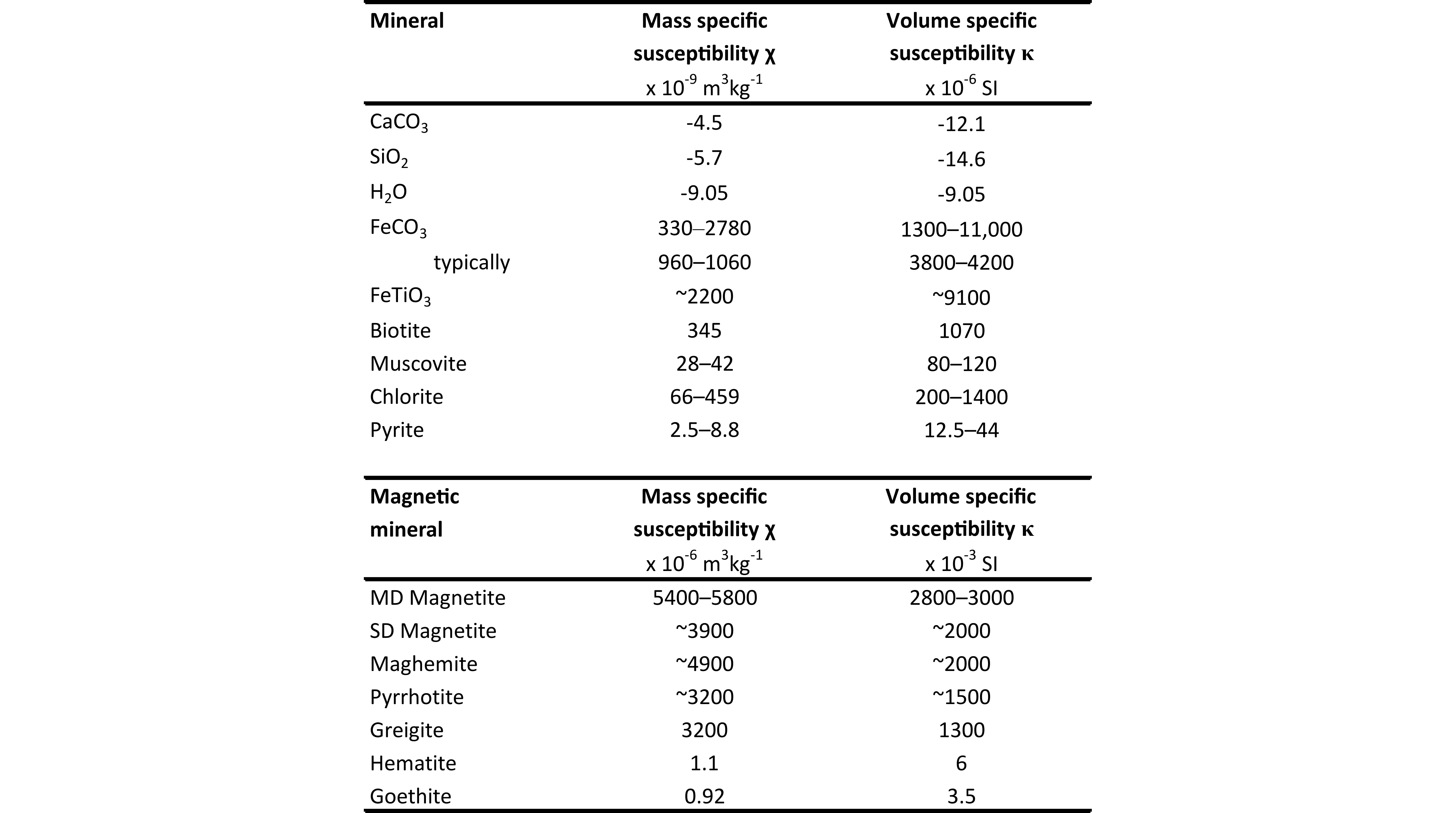
15When all orbitals in a compound are filled with electrons (each with one spin-up and one spin-down electron) such a compound is diamagnetic, for example quartz (SiO₂) is diamagnetic. When placed in a magnetic field the substance repels the field, it tries to undo the action of the field. Therefore, it has a negative magnetic susceptibility: its magnetic moment is directed opposite to the applied field. In a magnetic field the apparent weight of a diamagnetic substance becomes smaller. Since mass is a fundamental material property, it cannot change and the change in weight is due to an apparent reduction of the specific density of the material, ρ. Therefore, the unit of χ, the mass-specific-susceptibility, is [m³ kg^-1], the inverse of ρ [kg m^-3]. Diamagnetism is linear with applied field and independent of temperature (because in atomic orbitals the energy level between the ground state and excited states is large). Diamagnetism is a property of all orbitals and only macroscopically measurable in absence of all other magnetism contributions. Examples include calcite (CaCO₃), quartz, and water whose values are listed in Table 1.

Table 1. Magnetic susceptibility of some minerals at room temperature.

Sources. Calcite: Schmidt et al. (2006). Quartz: Hunt et al. (1995). Water: Philo & Fairbank (1980). Siderite: Hunt et al. (1995), Rochette et al. (1992). Ilmenite: Cui et al. (2002). Biotite, muscovite, chlorite: Martin-Hernandez & Hirt (2003). Pyrite: Burgardt & Seehra (1977). Magnetite, maghemite, pyrrhotite, hematite: Borradaile & Henry (1997). Greigite: Roberts et al. (2011).

1.3. Paramagnetism

16When there are one or more free electrons in one or more orbitals, i.e. electrons with uncompensated spins that are not coupled over inter-atomic distances, paramagnetism results. Free spin electrons tend to align with an applied field because then their energy is minimized. The aligning tendency is opposed by the randomizing effect of temperature. Classic Curie-Weiss paramagnetism is inversely correlated with absolute temperature, according to the law named in their honor (e.g. Cullity & Graham, 2008).

17 M = χH = ^C/_T H (3)

18where C is the Curie constant, a material property related to its constituting ions’ magnetic moments, and T the absolute temperature. A paramagnetic substance gains apparent weight in an applied field.

19The field dependence of paramagnetism is described with the Langevin function (e.g. Tauxe et al., 2018). At room temperature paramagnetism is linear with the applied field up to fields of several hundreds of Tesla. Technically such high magnetic fields are very difficult to generate, only possible in a few dedicated facilities world-wide (Dresden (Germany), Grenoble and Toulouse (France), Nijmegen (The Netherlands), Hefei (China), and Tallahassee (USA)). Static hybrid magnets (combinations of superconducting and resistive (electromagnetic) magnets) can reach fields up to 45 Tesla and pulse magnets up to ~100 Tesla. At very low temperatures, say below 20 Kelvin, paramagnetism may saturate in applied fields of a few Tesla only. At low temperatures the field dependence is described by the so-called Brillouin function which considers a finite number of atomic energy levels dictated by quantum mechanical considerations. A Langevin function considers all energy levels which is a good approximation at high temperatures, room temperature and above.

20The susceptibility of a paramagnet is primarily governed by its iron content; its manganese content plays a secondary role. Thus, minerals like ilmenite (FeTiO₃) and siderite (FeCO₃) have high susceptibility values (see Table 1). For most rock-forming paramagnetic minerals a susceptibility range is quoted, depending on their amounts of substituted iron and (to a lesser extent) manganese. It should be kept in mind that inclusions of (titano)magnetite (a solid solution between the end members magnetite (Fe₃O₄) and ulvöspinel (Fe₂TiO₄)) and other magnetic minerals may have their bearing on magnetic susceptibility ascribed to silicates (e.g. Martín-Hernández & Hirt, 2003; Borradaile & Werner, 1994).

21Two more special types of paramagnetism deserve brief mentioning here: Pauli paramagnetism and Van Vleck paramagnetism, both essentially independent of temperature in contrast to Curie-Weiss paramagnetism. They arise from quantum mechanical effects of electron spin interaction. Because spins tend to align with an applied magnetic field both Pauli and Van Vleck paramagnets have small positive susceptibility, typically an order of magnitude lower than Curie-Weiss paramagnets (Mugiraneza & Hallas, 2022). Pauli paramagnetism is largely confined to metals and as such not that relevant in geoscience. A foremost example of Van Vleck paramagnetism includes pyrite (FeS₂) (Burgardt & Seehra, 1977) which is the most common sulfide in a variety of sedimentary rocks.

1.4. Ferromagnetism sensu lato

22Coupling of electron spins over interatomic distances results in macroscopic magnetism: ferromagnetism, ferrimagnetism, or antiferromagnetism. Ferro- and ferrimagnets typically have a high magnetic susceptibility while that of antiferromagnets lies in the range of paramagnetic materials. Data for common minerals are compiled in Table 1. Traces of ferro- or ferrimagnetic minerals thus may dominate the bulk susceptibility of rocks. But caution should be taken to take susceptibility as direct measure of magnetic mineral content, particularly for rocks with weak magnetic susceptibility.

23As is well known, ferrimagnetic particles, with magnetite as the foremost example, show magnetic properties that are grain-size dependent. Large grains with sizes beyond ~10–20 μm (numbers refer to room temperature values) are multidomain (MD) and equant grains between ~30–80 nm are single domain (SD). Grains between those sizes are classically referred to as pseudo-single-domain (PSD) (e.g. Dunlop & Özdemir, 1997) and have been imaged to contain non-collinearly coupled spins in vortex structures (Harrison et al., 2002). With increasing grain size, the traditional PSD range is divided into the flower state, single vortex, and multi-vortex states before grains with a few domains prevail (Roberts et al., 2017). The transitions between those states are gradual and sizes depend on the shape, presence of intergrowths, and strain state of the particles. Also, the lower boundary of ‘true MD’ particles with many magnetic domains is not sharp.

24For large spherical MD grains, the theoretical maximum volume susceptibility is 3, i.e. 1/N with N the demagnetization factor (N = 1/3 for a sphere, e.g. Dunlop & Özdemir, 1997). Measured values (see Table 1) are close to that limit. SD particles have a lower susceptibility than MD particles because it is more difficult in low applied magnetic fields to rotate the coupled electron spins than to translate a domain wall. The volume susceptibility of SD particles is

25κ_SD = 2M_s/3H_k (4)

26M_s the spontaneous magnetization and H_k the microscopic coercive force. For a uniaxial SD particle collection H_k = 2.09H_c with H_c denoting the macroscopic coercive force (Hrouda, 2011).

27Particles with sizes smaller than 30 nm, the lower boundary of the SD realm at room temperature, are superparamagnetic (SP): they cannot retain a stable remanent magnetization, but they possess a coupled electron spin structure. This results in a very high susceptibility, substantially higher than the susceptibility of bulk material of that mineral. Through the SP grain-size range, the relaxation time τ of the coupled spins, a concept introduced by Néel (1949), increases from the atomic time scale (~10^-9 s) to the geological time scale (10⁺⁹ year) at ~30 nm. The relaxation time is given by:

28τ = τ₀e^(KV/kT) (5)

29with τ₀ being the atomic reorganization time (~10^-9 s), K the anisotropy constant at the temperature of interest, V the particle volume, k the Boltzmann constant, and T the absolute temperature.

30Instrumental time scale is often defined at a relaxation time of 100 s, corresponding to ~25 nm for an equant particle. From 0 to 30 nm the volume susceptibility increases linearly with the number of coupled spins, i.e. volume, from paramagnetic values up to very high numbers according to:

31κ_SP = μ₀V(M_s)²/3kT (6)

32where μ₀ = permeability of vacuum, V = particle volume, k = Boltzmann’s constant and T absolute temperature.

33Because an SP particle’s relaxation time is in the instrumental time scale range, a distribution of SP particles can be sensed through the measurement of their susceptibility at various frequencies. For a given frequency, say 960 Hz (typical of an MFK family susceptometer), a set of particles is SP when the measurement frequency is lower than the relaxation time of the particle collection, so the collection behaves as a paramagnet by following the applied field. For the 15.6 kHz frequency of the instrument the particle set may be SD when the measurement frequency is higher than the corresponding relaxation time (Néel, 1949), so the particle collection is ‘locked’ with respect to the applied field and behaves like an SD particle collection. Thus, at a given temperature the low-frequency susceptibility is higher than the high-frequency susceptibility.

34The blocking volume V_B, at which a particle transitions from SP to SD, thus depends on the measurement frequency and is expressed by (e.g. Schneider et al., 2025):

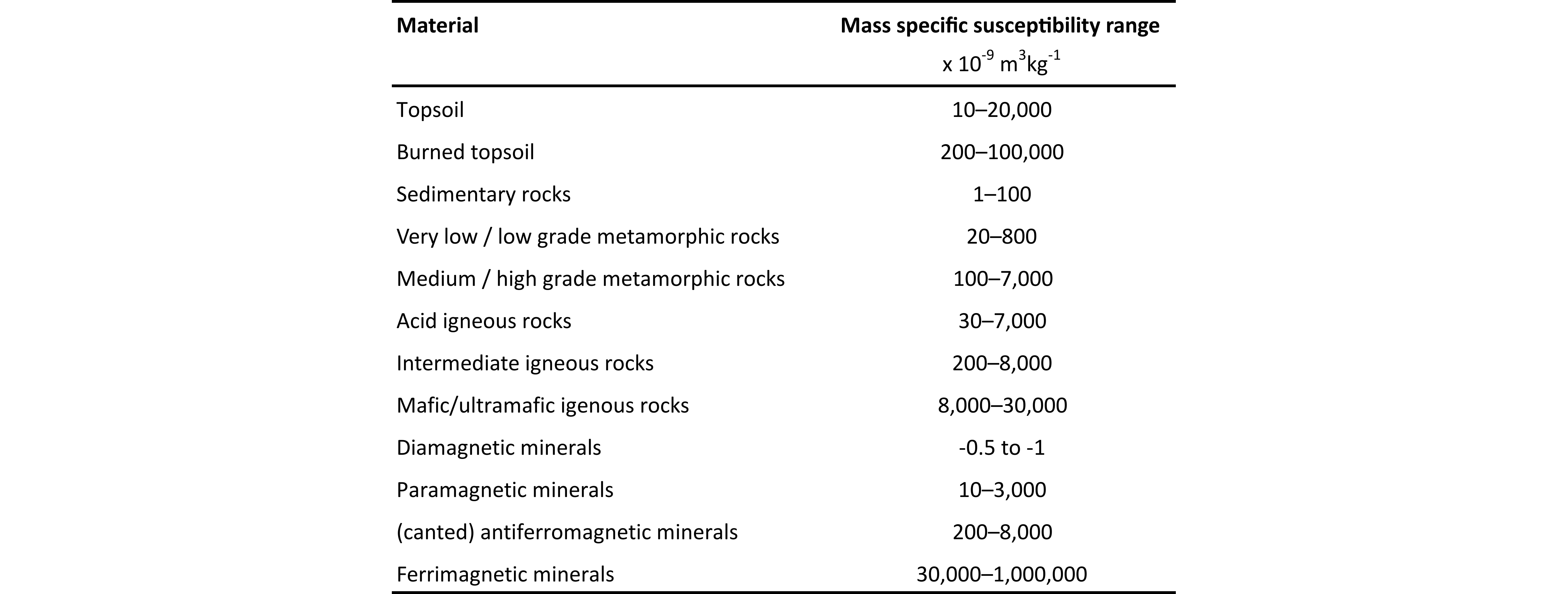
35V_B = -(2kT/μ₀H_kM_s).ln(2πfτ₀) (7)

36with 2πfτ₀ corresponding to the measurement time for the measurement frequency f for the blocking relaxation time τ₀.

37The frequency dependence may be expressed as the difference between the susceptibilities (e.g. Dearing et al., 1996):

38κ_(freq) = κ_(lowfreq) – κ_(highfreq) (8)

39as a percentage (typically used)

40κ_(freq%) = 100%*((κ_(lowfreq) – κ_(highfreq))/κ_(lowfreq)) (9)

41It should be realized that κ_(freq%) is dependent on the operating frequencies (e.g. Hällberg et al., 2020). Therefore, either normalizing to a decadal frequency difference should be done or the normalized frequency dependence, κ_FN (Hrouda, 2011) should be used (this is less often done)

42κ_FN = κ_(freq%).ln(κ_(highfreq)/κ_(lowfreq)). (10)

43An implicit assumption in these calculations (equations 9 and 10) is that the measured susceptibility is residing in ferromagnetic particles since diamagnetism and paramagnetism do not show frequency dependent susceptibility. Hence, when the rocks under investigation have a high diamagnetic or paramagnetic contribution resulting in a low or even negative susceptibility, this assumption may break down and the true amount of SP particles is underestimated when the frequency dependence is expressed as a percentage as for example recently noted by Bradák et al. (2021) in their study on European loess sequences or Gallo et al. (2025) who work in their study on remagnetized Ediacaran rocks from Paraguay with the ‘absolute’ frequency dependence (equation 8), which is directly related to the amount of SP particles.

44Here also the imaginary, quadrature, or out-of-phase susceptibility κ” deserves mentioning. It is 90° out of phase with the applied field and represents the energy loss and time-dependent magnetization delay (e.g., Mullins & Tite, 1973). For SP particles it is largest for particles just below their blocking volume for a given temperature (Hrouda et al., 2013). To calculate f_D(D_(b,i)), the total volume of the particles with diameters straddling 1 nm around a given blocking volume V_B from the out-of-phase susceptibility, Jonsson et al. (1997) demonstrate this approximation for the blocking volume

45f_D(D_(b,i)) ≈ (9/π).[(B_K)/µ₀M_sD_(b,i)].κ”(f,T_i) (11)

46with B_K = µ₀H_K, D_(b,i) = (6V_B/π)^1/3, the particle diameter corresponding to the blocking volume V_B at a given frequency and temperature, and M_s the saturation magnetization at the respective temperature.

47Since the out‐of‐phase magnetic susceptibility and the frequency dependence of the in‐phase component are proportional (Néel, 1949; Hrouda et al., 2013), also called the π/2‐law, κ” in equation 11 can be replaced with κ_FN π/2, with κ_FN from equation 10 (Egli, 2009). Thus, magnetic particle size distributions can also be obtained from in‐phase susceptibility component measurement in a directly analogous manner to the out-of-phase susceptibility measurement.

48The low-field susceptibility of ferromagnets is implicitly taken as linear with applied field. This is correct for very low, earth-like fields. Importantly, the sample’s magnetic behavior is fully reversible: by measuring the susceptibility (or its AMS) the magnetic state of that sample is not changed. However, in higher fields the magnetic response of ferromagnets is more complex; in fields slightly larger than the linear susceptibility domain the sample’s magnetic moment M increases over-proportionally and is described with:

49M = κH + γH² (12)

50The quadratic term γH² is associated with Barkhausen jumps of domain walls where γ is a material property describing the field dependence of domain wall motion. The equation was derived by Lord Rayleigh in 1887 and the field realm where it is valid is therefore referred to as the Rayleigh domain. After removing the (small!) field the domain walls relax to their original position; the sample’s magnetic behavior is still reversible. Natural magnetic minerals are in the linear domain for typical susceptometer field ranges, only pyrrhotite (Fe₇S₈-Fe₁₁S₁₂) may already be in the Rayleigh domain, a feature proposed to establish the presence of pyrrhotite through susceptibility measurements at various small fields (Hrouda et al., 2006). For stronger fields, beyond the Rayleigh domain, samples show magnetic hysteresis upon cycling in a field. When subjecting a sample to a loop starting at positive field, slowly going to the same negative (= oppositely directed) field, and then back to the same positive field, its magnetic moment shows a loop, the magnetic hysteresis loop. Loops in fields where magnetic saturation is not reached are called minor loops and loops in saturating fields are major loops. After hysteresis loop measurement the magnetic state of a sample has changed. The susceptibility measured in a single sample before and after hysteresis loop measurement may well have changed.

1.5. Instruments for susceptibility measurement

51Instruments for measuring low-field susceptibility and its anisotropy are often bridge-type instruments where the imbalance induced by the sample between a pair of coils in an oscillating field induced by an alternating current (AC) is measured and via a calibration sample is transferred to a susceptibility value. Measurement frequency varies between a few hundreds to a few tens of thousands Hz and measurement fields between a few A/m to ~800 A/m. Magnetic Property Measurement System (MPMS) instruments use SQUID (Superconducting QUantum Interference Device) sensors to measure susceptibility. Sometimes the slope of the major hysteresis loop at zero field is taken as approximation of the low-field susceptibility although this is strictly speaking incorrect. Commercially available AC-susceptometers which can measure at several frequencies include the Bartington MS2/MS3 susceptometer (470 Hz, 4.7 kHz; Bartington instruments (Oxon, UK)) and the MFK1 and MFK2 susceptometers (976 Hz, 3.9 kHz, 15.6 kHz, AGICO, Brno Czech Republic)). In their recent study of susceptibility and its frequency-dependence in a Late Quaternary Tajikistan loess-paleosol sequence Schneider et al. (2025) employ a DynoMag instrument (variable frequency from 1 Hz to 500 kHz, RISE magnetic sensors inc. (Gothenburg, Sweden)) to measure the susceptibility at 15 frequencies—termed multi-frequency magnetic susceptibility analysis by those authors—which enables a detailed assessment of the grain-size distribution within the SP realm following Maher (2007), Hrouda (2011), and Hrouda et al. (2013). Out-of-phase susceptibility can be measured amongst others with MPMS style instruments (Quantum Design, San Diego, USA), the aforementioned DynoMag instrument, and the KLY5 (AGICO, Brno, Czech Republic).

2. Susceptibility in rocks

52The susceptibility ranges of common rock types (Table 2) vary substantially but also overlap. Mafic igneous rocks have highest susceptibility and sediments the lowest since mafic rocks typically contain a fair of magnetite. The susceptibility range of sediments overlaps with that of a variety of metamorphic rocks. The variation of susceptibility in stratigraphic sequences of sediments is traditionally interpreted as a depositional signature so that a record can be taken as a climate proxy, primarily reflecting rainfall variability in continental sediments (e.g. Maher & Thompson, 1995; Ellwood et al., 2000). In marine settings higher rainfall is associated with higher continental runoff delivering more clastic sediments typically leading to a (slightly) higher susceptibility. This is a good starting approach when working with unconsolidated sediments. However, the potential presence of magnetofossils (the magnetic remnants of magnetotactic bacteria that form magnetic particles within their cells) that form in-situ should not be overlooked in marine and lacustrine sediments, also when dealing with sediments with a terrigenous provenance as illustrated for example by Just et al. (2012) in tropical Atlantic sediments off-coast Gambia or by Yamazaki & Ikehara (2012) in Southern Ocean sediments. More recent examples include Usui et al. (2017) and Li et al. (2022). Magnetite (e.g. Blakemore, 1975) and greigite (Fe₃S₄, e.g. Mann et al., 1990) magnetofossils are known. Conditions favoring the occurrence of magnetotactic bacteria are likely (paleo)climatically related, justifying the use of the magnetic susceptibility as paleoclimate proxy but source-to-sink analyses may be biased by not properly recognizing the magnetofossil contribution that is formed in situ at the depositional site. In lithified sediments the effects of diagenesis and burial may play up. To better appreciate such effects, we review next how early diagenesis, late diagenesis, and burial may influence the susceptibility of a rock. Dissolution or formation of ferrimagnetic minerals may have an appreciable effect.

Table 2. Mass specific susceptibility ranges of soils, common rocks, and minerals.

Data from Dearing (1999).

2.1. Burial: Impact of diagenesis and metamorphism

53After deposition a sediment is subjected to the rock cycle starting with burial which inevitably comes with diagenesis. Early diagenesis starts shortly after sediment deposition and may involve the formation of magnetofossils and/or inorganically formed greigite. Late diagenesis occurs during deeper burial and when buried sufficiently deep, the rocks become metamorphic. A myriad of diagenetic reactions is possible depending on the sediment and the diagenetic conditions. Many involve either the breakdown or the formation of magnetic minerals with evident impact on the susceptibility of such rocks. Next to the potential impact of magnetotactic bacteria that should be assessed on a case-by-case basis, the rule of thumb for unconsolidated sediments: “more clastic material = higher low-field susceptibility” may break down.

54Early vs late diagenesis crudely follows the distinction between soft and lithified sediments but is only loosely constrained by time and temperature (Roberts, 2015). They are also referred to as syn-diagenetic and ana-diagenetic as defined by Fairbridge (1967) who distinguishes also epi-diagenetic reactions, i.e. late diagenetic reactions during uplift of a sedimentary succession. In terms of magnetic mineralogy Aubourg et al. (2012) and Kars et al. (2014) distinguish three diagenetic zones or windows depending on the burial temperature: the greigite window at low temperatures below ~50 °C, the magnetite window at intermediate temperatures roughly between 60 and 150 °C, and the pyrrhotite window at the highest diagenetic temperatures starting at ~150 °C and extending into the metamorphic realm. The temperatures are loosely defined and a large overlap between adjacent zones exists. Clastic and biogenic magnetite may survive the greigite window (Aubourg et al., 2012; Kars et al., 2014).

55Ferrimagnetic greigite, magnetite, and pyrrhotite have a high low-field susceptibility (Table 1), so their formation (or breakdown) interferes with assigning a depositional signature to a susceptibility record without further constraints. Trace amounts of these magnetic minerals may constitute an appreciable portion of the bulk susceptibility of the sediment. This is illustrated in Figure 1, a numerical simulation of a sediment, a ‘calcite / typical paramagnet’ mixture, with a constant amount of magnetite added. For magnetite amounts >1 per mil, the bulk susceptibility of the rock can confidently be equated to the amount of magnetite but for lower magnetite amounts, for example typical of many pelagic sediments, this is not the case. For magnetite amounts <100 ppm, diagenetic addition (or removal) of several tens of ppm magnetite (or greigite or pyrrhotite which have similar high susceptibility) determines the bulk susceptibility of the rock. This notion should be considered when interpreting susceptibility records of a sedimentary succession. Next to bulk susceptibility measurements, additional rock magnetic measurements on selected samples may include hysteresis loops and first-order-reversal curve diagrams (e.g. Tauxe et al., 2018; Roberts, 2026), coercivity component analysis of acquisition curves of the isothermal remanent magnetization (IRM) (Kruiver et al., 2001; Egli, 2004; Maxbauer et al., 2016) and thermal demagnetization of distinct IRM coercivity fractions imparted orthogonally (Lowrie, 1990).

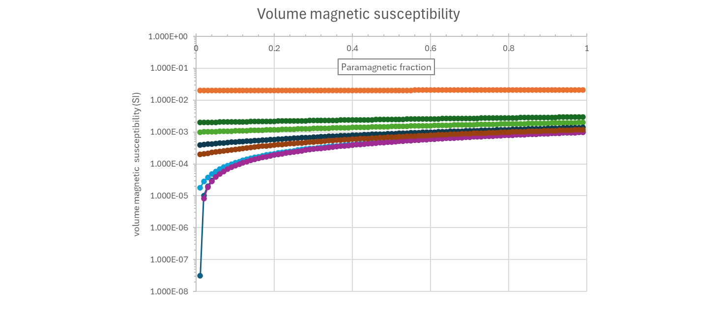
Figure 1. Numerical simulation of the volume susceptibility of a diamagnetic-paramagnetic mixture (calcite and typical paramagnet) with a constant amount of magnetite added. Note the logarithmic ordinate scale. Purple: diamagnetic-paramagnetic mixture without magnetite (negative numbers cannot be displayed logarithmically so the curve stops at 0.02); dark blue: 1 ppm magnetite; light blue: 10 ppm magnetite; brown: 100 ppm magnetite; dark green: 200 ppm magnetite; light green: 500 ppm magnetite; intermediate green: 1000 ppm magnetite; orange: 1% magnetite. For magnetite contents >1 per mil the bulk susceptibility of the (simulated) rock can be equated to the amount of magnetite.

56We now summarize the impact of diagenetic reactions on the magnetic minerals starting with the ambient temperature, early diagenetic processes. Magnetosomes form under appropriate conditions in many sedimentary settings. Bacteria with SD magnetite crystals within their cells, named magnetosomes, were discovered in recent sediments by Blakemore in 1975 (Blakemore, 1975). They also occur in soils (Fassbinder et al., 1990). Magnetotactic bacteria with SD greigite magnetosomes were discovered later, in 1990 (Farina et al., 1990; Mann et al., 1990). Their survival over geological time scales was debated initially but magnetosomes in sediment successions of at least Cenozoic and Mesozoic ages have been convincingly demonstrated (e.g. Chang & Kirschvink, 1989; Kopp & Kirschvink, 2008; Vasiliev et al., 2008). While the presence of magnetofossils in slowly accumulating pelagic settings is known since the 1980s (e.g. Kirschvink & Chang, 1984), in sediments with a dominant terrigenous input their contribution to magnetic signal was deemed low until the early 2010s. More recent studies have shown their omnipresence in variable amounts in essentially all sedimentary settings, and also in lithified sediments. This pertains to both magnetite and greigite magnetofossils.

57Greigite—until recently considered a metastable phase in the pyrite formation reaction chain—is thermodynamically stable under certain Eh-pH conditions (Rickard et al., 2024). In the presence of reactive iron, inorganic diagenetic greigite formation is associated with the availability of organic matter and sulfide (Kao et al., 2004). When dissolved reduced sulfur (HS^-) is available in limited amounts like in fresh water and estuarine sediments affected by early diagenesis, greigite is dominant and pyrite only subordinate. When reduced sulfur is plentiful like in marine sediments undergoing early diagenesis, pyrite is very dominant but traces of greigite may occur (Roberts, 2015). Greigite may grow in several mineral associations. Roberts & Weaver (2005) list five dominant modes of occurrence but do not exclude others: (1) the surface of early diagenetic framboidal and nodular pyrite, (2) within cleavages of detrital sheet silicate grains, (3) the surfaces of authigenic clays, (4) the surface of siderite, and (5) the surface of gypsum (previously oxidized nodular pyrite). Modes 4 and 5 are less common than modes 1–3. When greigite forms shortly after sedimentation, i.e. quasi syn-sedimentary within 5–10 kyr, trustworthy magnetostratigraphic correlations with the Geomagnetic Polarity Time Scale (GPTS) are possible (e.g. Vasiliev et al., 2008; Hüsing et al., 2009; Kelder et al., 2018). However, greigite may form as well during later stages in the geological history of a sediment, complicating magnetostratigraphic interpretations (e.g. Sagnotti et al., 2010; Aben et al., 2014). Early diagenetic pyrrhotite is rare and typically occurs as rosettes or sheaf-like bundles (Dinarès-Turell & Dekkers, 1999). An association with gas-hydrate conditions is suggested by Larrasoaña et al. (2007).

58Diagenetically enriched greigite-bearing strata have higher susceptibility than other sediments. The amount of organic matter could be related to climate, i.e. depositional conditions, but a one-to-one relationship between the greigite content and organic matter does not exist, compromising direct interpretation of a susceptibility record in terms of depositional conditions. The same goes for diagenetic pyrite which often forms at the expense of magnetic minerals; thus, pyrite formation lowers a sediment’s susceptibility. An example includes the pyrite enriched zones below sapropels in Mediterranean sediments (e.g. Passier et al., 2001; Larrasoaña et al., 2003).

59Magnetite may be forming diagenetically at burial depths >2 km leading to pervasive remagnetization. Useful reviews include McCabe & Elmore (1989), Jackson & Swanson-Hysell (2012), and Van der Voo & Torsvik (2012). Earlier proposed remagnetization scenarios involved large amounts of externally derived ‘basinal’ fluids related to orogenic action (Oliver, 1986). The occurrence of low-temperature, so-called Mississippi Valley Type, lead-zinc ores and hydrocarbon accumulation was also inferred to be related to such fluids. Later the role of such external fluids for orogen-wide pervasive remagnetization is downplayed because their volume is only limited (Jackson & Swanson-Hysell, 2012; Van der Voo & Torsvik, 2012). Internally buffered fluid scenarios are much more likely. Iron released by the smectite-to-illite reaction occurring between ~70–140 °C is often deemed the source of the magnetite (e.g. Lu et al., 1990; Banerjee et al., 1997; Katz et al., 2000; Tohver et al., 2008). Also pyrite oxidation (e.g. McCabe et al., 1983; Suk et al., 1990a, b; Weil & Van der Voo, 2002; Zwing et al., 2005; Huang et al., 2015) or pressure solution have been proposed as mechanism (e.g. Zegers et al., 2003; Elmore et al., 2006; Oliva-Urcia et al., 2008). Integration of magnetic property research with (electron) microscopy, X-ray diffraction, and structural analysis is recommended (e.g. Jackson & Swanson-Hysell, 2012). Remagnetized carbonates show distinctive magnetic properties due to authigenic magnetite grains dominantly in the SP-SD size range, often referred to as the ‘fingerprint’ of remagnetization (Jackson & Swanson-Hysell, 2012). These are ‘wasp-waisted’ hysteresis loops, high ratios of anhysteretic remanent magnetization to saturation remanent magnetization, and a high frequency-dependence of susceptibility. Magnetite formation mechanisms are bound to vary spatially and temporally within and between orogens and which mechanism(s) was(were) active should be ascertained in each target section. Sr isotope ratios close to the coeval seawater ratio points to internally buffered magnetite growth. Stable carbon and oxygen isotopes, and trace element signatures can also be utilized to explore potential magnetite formation pathways (Katz et al., 2000; Zwing et al., 2005). In a recent study using statistical learning techniques Gallo et al. (2025) also concluded that isochemical remagnetization prevailed in their Ediacaran carbonate rocks from Paraguay.

60Here we focus on the potential impact on a susceptibility record. In case of a direct magnetite-clay mineral association the susceptibility record may still reflect a depositional signature, even with a possibly enhanced susceptibility contrast between ‘high’ and ‘low’ susceptibility strata because of the formation of trace amounts of ferrimagnetic magnetite in the former. However, when this direct association is lost, a susceptibility record cannot be interpreted anymore along depositional lines. It remains to be investigated, however, at which temperature and geochemical conditions the direct linkage becomes tenuous. This has immediate bearing on cyclostratigraphic reconstructions in deep time; the suitability of target sections should be ascertained on a case-by-case basis. An example will be given later.

61Pyrrhotite forms deeper than c. 6 km in sediments starting at temperatures close to ~150–200 °C (e.g. Aubourg et al., 2012). Aubourg et al. (2019) argue for the formation of fine-grained pyrrhotite starting already at 60 °C. Late diagenetic, synfolding pyrrhotite formation in early Miocene sediments from Sakhalin has been reported by Weaver et al. (2002). Pyrrhotite may form at the expense of magnetite at ~250 °C and of pyrite at >350 °C (Rochette & Lamarche 1986; Rochette, 1987; Crouzet et al., 2001; Schill et al., 2002). It is generally associated with unambiguously remagnetized rocks (e.g. Zegers et al., 2003; Weil et al., 2010; Van der Voo & Torsvik, 2012; Pastor-Galán et al., 2015). However, intricacies of formation pathways have yet to be explored.

62Thus, for a proper interpretation of a susceptibility record, the susceptibility carrier should be known. This implies that one should have supporting rock magnetic information, an often underappreciated aspect. Next some examples of magnetic susceptibility records and their interpretation will be discussed.

3. Applications in geoscience

63The success of susceptibility as a proxy for paleoclimate and its power as a duration chronometer for high resolution time scale construction is illustrated next. The second group of studies, discussed in section 3.2, relies in particular on recognizing orbital frequencies in a susceptibility record.

3.1. Susceptibility in loess-paleosol sequences as a hydroclimate indicator

64Up to the early 1980s the age of the vast and thick loess-paleosol sequences on the Chinese Loess Plateau (CLP) was only loosely constrained and heavily debated. With the landmark publication by Heller & Liu (1982) this changed completely: by demonstrating magnetostratigraphy as a robust dating tool for this purpose they showed that loess-paleosol sequences were considerably older than thought before and spanned the entire Quaternary. They also showed that the loess/paleosol susceptibility and the Marine Isotope Stage (MIS) records exhibit essentially the same pattern indicating the paleoclimate potential of susceptibility records in loess/paleosol sequences. This was setting the stage for thousands of papers on loess-paleosols on the CLP and elsewhere. On the CLP, paleosols have a higher magnetic susceptibility than the intervening loess and their expression is more pronounced to the SE of the plateau which features higher rainfall under the influence of the Asian Summer Monsoon. Close correlation to MIS with paleosols correlating to warm and wet periods was demonstrated first for young loess-paleosols (e.g. An et al., 1991) but later also for much older records extending into the underlying red clay sequences (e.g. Sun et al., 1998; Sun et al., 2006; Maher, 2007, 2011, 2016; Ao et al., 2016, 2024). Susceptibility is thus a powerful proxy for summer monsoon activity as illustrated next.

65Through comparing magnetic susceptibility fluxes with ¹⁰Be fluxes Heller et al. (1993) demonstrate that in-situ production of magnetite (sensu lato) was essentially halted during loess deposition and enhanced during interglacial times. They show a linear correlation between pedogenic flux and paleorainfall. Maher et al. (1994) use the modern rainfall trend to calibrate magnetic susceptibility enhancement. They empirically defined the relation between rainfall and susceptibility, termed climofunction by them:

66Annual precipitation (mm/yr) = 222 + 199 log χ(B-horizon – C-horizon) (13)

67The B-horizon (sometimes also referred to as subsoil) is the zone of illuviation in which material leached from the A-horizon (or topsoil) is accumulating. The C-horizon, below the B-horizon, is incipiently physically weathered parent material.

68A much larger paleorainfall variability across the CLP was found than anticipated beforehand. Maher (2016), in her compilation, provides more data supporting the calibration (Fig. 2), caution for similar paleosol conditions for the relation to work, and show that for rainfall beyond ~1000–1200 mm/yr the trend line breaks down. Balsam et al. (2011) caution for local variability in the paleosol vs precipitation trend and demonstrate that inclusion of more independent variables (obtained with diffuse reflectance spectroscopy (DRS), X-ray diffraction (XRD), or X-ray fluorescence (XRF) analysis) in their multiple regression markedly improves the correlation. For precipitation less than ~200 mm/yr the susceptibility enhancement vs rainfall relation breaks down (Balsam et al., 2011). Based on more extended magnetic property data sets, susceptibility vs precipitation trends were found for example by Panaiotu et al. (2001) for Romanian loess-paleosols and Geiss et al. (2008) for North American loess-paleosols.

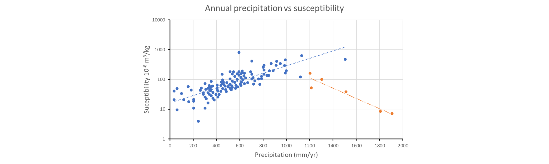
Figure 2. Susceptibility vs annual precipitation for recent soils, redrawn with data compiled by Maher (2016). With increasing precipitation up to ~1000 mm per year the susceptibility goes up (blue trendline) because of increasing pedogenesis. Beyond ~1000 mm per year susceptibility goes down (orange trendline) with increasing precipitation because waterlogging effects play up. Loess-paleosol differences appear to be reflected in different ways depending on their location. Already in the 1990s, two main models were developed to explain the enhancement of magnetic susceptibility (e.g. Forster et al., 1994; Evans & Heller, 1994; Evans, 2001): the pedogenic enhancement and wind vigor models, reviewed for example by Maher (2016). The former typifies most CLP loess-paleosol sequences where paleosols have higher susceptibility and higher frequency dependence of susceptibility than intervening loess portions due to enhanced pedogenesis. This pedogenic enhancement can be fitted with a linear trend between susceptibility and its frequency dependence conveniently named the “true loess line” by Zeeden et al. (2016) but already generally used since the 1990s.

69However, as originally observed in Alaska (Begét & Hawkins, 1989) and found subsequently elsewhere as well, loess has a higher susceptibility than intervening paleosols. This was explained by the enrichment of coarse-grained magnetite in loess over paleosols due to the action of surface winds during glacials: stronger winds enable entrainment of coarser particles (Evans, 2001). Yet while the loess has a higher susceptibility, intervening paleosols show higher frequency dependence as demonstrated by Bidegain et al. (2005) for pampa loess in Argentina and Kravchinsky et al. (2008) for Siberian loess-paleosol sequences. This indicates pedogenic neoformation of SP magnetite or maghemite particles also in those sequences.

70The role of water logging should be assessed as well in this context (Maher, 2011; Zeeden et al., 2018). In a plot of the low frequency susceptibility vs the absolute frequency dependence (placed on a common frequency interval) wind vigor tends to lower the frequency dependence for a given susceptibility placing influenced loess-paleosol sequences above the ‘true loess line’. Water logging dissolves magnetic minerals lowering their susceptibility. Yet, before complete dissolution the finest, SP, particles raise the frequency dependence (Fig. 3).

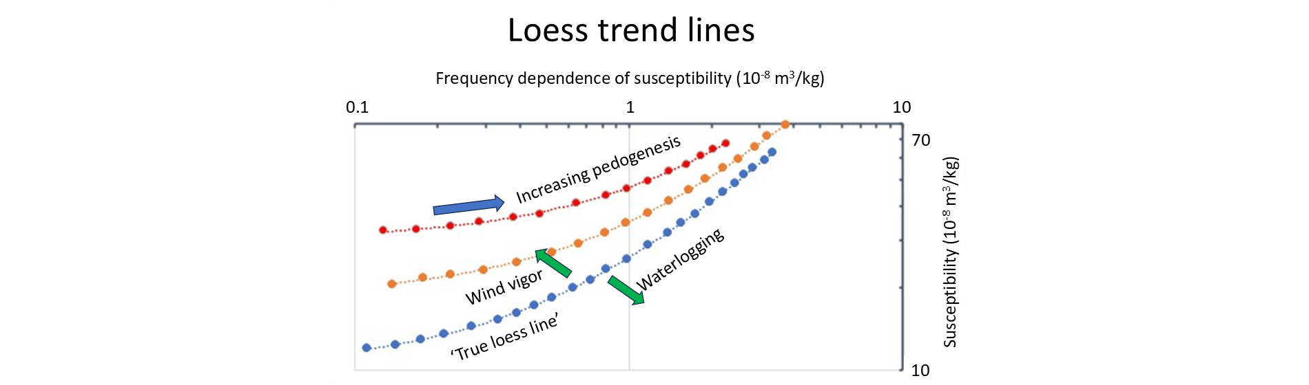
Figure 3. Susceptibility-frequency dependence of susceptibility trendlines (redrawn from Bradák et al., 2021). The frequency dependence is placed on a common frequency difference following Hrouda (2011). The leftmost points indicate the background susceptibility for a given location with increasing pedogenesis to the upper right for the respective trendlines. The ‘True loess line’ is the pedogenic enhancement model from the Chinese Loess Plateau. The orange and red trendlines are from the middle and lower Danube Basin respectively (Újvári et al., 2016; Zeeden et al., 2018). Wind vigor decreases the frequency dependence and waterlogging reduces the susceptibility while increasing its frequency dependence.

71Bradák et al. (2021) and Zeeden et al. (2018) studying European loess-paleosol sections noted potential surface oxidation of magnetite impacting the data. Such oxidation is also possible in the loess source areas, as shown by Van Velzen & Dekkers (1999) and confirmed by Spassov et al. (2003) for CLP sections. However, heating samples at 150 °C and measuring the samples’ magnetic properties again afterward, documented by Van Velzen & Dekkers (1999) as tool to detect the phenomenon, was not performed by Bradák et al. (2021) and Zeeden et al. (2018). Surface oxidation is manifested by a decrease in coercivity of up to 40% after annealing at 150 °C, while susceptibility shows a moderate increase or decrease up to 10% (Van Velzen & Zijderveld, 1995). Upon stress relaxation, the susceptibility is increasing because of the lower coercivity (Van Velzen & Zijderveld, 1995; Van Velzen & Dekkers, 1999). Decreasing susceptibility, also observed in loess and paleosols, may be related to the presence of fine SP particles, fully disordered after annealing (Van Velzen & Dekkers, 1999). The effect in loess samples is larger than in paleosols pointing to the importance of magnetite as pure endmember as maghemite (γ-Fe₂O₃) is already fully oxidized and cannot be affected by further oxidation. Also Schneider et al. (2025) point to prevalence of oxidized rims around magnetite grains as documented by exchange bias due to core-rim interaction (Spassov et al., 2024) which is more pronounced in loess than in paleosols in a Tajikistan section indicating ancient weathering in the loess source area. In situ formation of SP particles occurs in both loess and paleosols. This is in line with the findings of Ahmed & Maher (2018) that soil wetting-drying oscillations are dominant in the formation for fine-grained magnetite in CLP paleosols. Al-free maghemite is present in minor amounts which is negating a possible formation pathway via aluminous hematite that is present in soils (Ahmed & Maher, 2018). They also explain their observation with a ‘magnetite core / maghemitized rim’ model.

3.2. Cyclicity and time scale construction in deep time

72Improving the geological time scale for dating geological events and determining rates of change is a continuous effort of the geoscience community. In sediments the procedure is termed “Integrated stratigraphy”. Next to lithostratigraphy, increasing resolution is provided through sequence stratigraphy, biostratigraphy, magnetostratigraphy, and finally cyclostratigraphy (visually or based on proxies). These are all relative methods. Where possible, intercalated volcanic ash falls and lavas can be radiometrically dated to provide absolute ages to which successions can be anchored. However, the applicability of these methods reduces when going backward in time. Beyond the Mesozoic, reversals of the geomagnetic field are known but a GPTS is “under construction”. Biostratigraphy is a core technique in Phanerozoic strata; in Ediacaran strata diagnostic fossils are absent and further back in time fossils are hardly detectable, if present at all. However, sequences and cycles may be preserved regardless of the age of the rock succession. Biostratigraphy and magnetostratigraphy provide ~200 kyr to Myr scale resolution. Sequence stratigraphy using principles derived from the balance between sediment supply and accommodation space, has a variable resolution. First- and second-order sequences are typically attributed to eustatic changes induced by mantle convection and plate tectonics while 4th- through 6th-order sequences are due to orbitally controlled climate-change-induced eustatic variations (e.g. Boulila et al., 2011). Third-order sequences are increasingly attributed to long-period modulation cycles of eccentricity (which may vary between 1.2 and 2.4 Myr over geological time due to chaotic behavior of the solar system (see Laskar et al., 2011)) and obliquity (1.2 Myr) under icehouse conditions (e.g. Boulila et al., 2011).

73Sequence boundaries, however, cannot always be established unequivocally in outcrop sections while seismic lines are easier to interpret but need calibration from bore hole information (Simmons et al., 2020). The higher order sequences, often orbitally paced, are providing in principle a duration chronometer. This was realized early on by Ellwood and co-workers (e.g. Ellwood et al., 2000; Crick et al., 2001) who advocated the use of susceptibility as proxy in combination with spectral analysis for basin-wide and even global correlation. The latter may be over-ambitious without firm constraints from other disciplines because the local sea level trends may not be the same everywhere on Earth at the same time as basins may respond differently under the prevailing regional tectonic regimes (e.g. Simmons et al., 2020). Within a single basin, however, it may provide a powerful correlation tool. Longer increasing and decreasing trends in susceptibility are interpreted as eustatic regressive and transgressive features on top of which shorter cycles may be present (e.g. Ellwood et al., 2000; Crick et al., 2001). During icehouse periods, with large ice sheets developed on at least one pole, glacio-eustacy is the communis opinio accepted driver of short-term eustatic changes visible in the rock record but for warm, greenhouse periods without major glaciation on the poles, opinions differ: to explain the smaller eustacy effects, aquifer eustacy, thermo-eustacy, and minor glacio-eustacy action have been proposed (for a discussion, see e.g. Simmons et al., 2020).

74Depending on the depositional system very short cycles in the rock record, expressing for example solar cycles, are particularly prone to short-duration disturbances termed “environmental shredding” by Jerolmack & Paola (2010). Slumping, redeposition, and short-duration hiatuses, obscure potentially present high frequency cycles. Only in acknowledged continuous sedimentation settings, mostly (hemi)pelagic and deep marine environments, such short-duration cycles may be preserved in the rock record. Evidently the sampling density should be sufficient for their detection; the Nyquist frequency dictates at least two samples per target cyclicity.

75The spectral analysis approaches to infer potential orbital cyclicity have become increasingly sophisticated over the years. Today, the packages Acycle (Li et al., 2019) and Astrochron (Meyers, 2021) are commonly used. Their blindfold use, however, may result in over-confidence of determining ‘significant’ orbital cycles: the base line (the robust AR1 noise model) may impact the calculated spectral signature especially at low frequencies, and significance levels may lack proper statistical definition (Weedon, 2022; Smith, 2023). Integration with other spectral and statistical techniques, e.g. Continuous Wavelet Transform (CWT), Evolutive Harmonic Analysis (EHA), Average Spectral Misfit (ASM), and evolutionary correlation coefficients (eCOCO; Li M. et al., 2018), is recommended, and significance levels should be used with caution as supporting argument only (see e.g. the “false alarm level” and “false discovery rate” discussion in Weedon, 2022). The approach relies on recognizing the ‘orbital fingerprint’, the spectral ratio of the long eccentricity (405 kyr), short eccentricity (100–120 kyr), obliquity (41 kyr), precession (19–23 kyr; modern values for obliquity and precession), and possible combination tones in a proxy record in the depth domain or in the time domain if an age model constrained by biostratigraphy or magnetostratigraphy is available. The long eccentricity cycle is particularly robust, at least throughout the Phanerozoic, because it is determined by the resonance of the solar system while obliquity and precession become shorter when going back in time because the Moon is receding from Earth, reducing tidal dissipation (Berger et al., 1992; Laskar et al., 2004; Kent et al., 2018). When properly recognized this provides a precise chronometer. Particularly in case of visible cyclic patterns the approach finds manyfold application, also in deep time (e.g. Lantink et al., 2022). An example of the use of susceptibility records in this context is illustrated below.

76Da Silva et al. (2016) studied the limestone-rich strata of the Lower Devonian in the Prague Synform (Czech Republic). Susceptibility was measured in samples (sample resolution ~10–15 cm down to 5 cm in visually condensed portions of sections), from the three lowermost Devonian stages, the Lochkovian, Pragian and lower Emsian from two locations, Požár-CS (Lochkov and Praha formations), and Pod Barrandovem (Praha and Zlichov formations). A lower resolution Th-γ-ray record (~50 cm) was obtained from Branžovy (Praha Formation (Fm)). Spectral analysis was performed with the Astrochron package including the Continuous Wavelet Transform (CWT), Evolutive Harmonic Analysis (EHA), and Average Spectral Misfit (ASM) approaches. Da Silva et al. (2016) focused on the Lochkovian and Pragian which are complete. The Pragian was sampled at three locations; here the results from the Pod Barrandovem section, deep pelagic limestones, are reproduced (Fig. 4). Susceptibility is the primary proxy, supported by the (lower resolution) γ-ray record from Branžovy. The strata in the Prague Synform are remagnetized (e.g. Krs et al., 2001; Grabowski et al., 2008). In the Pod Barrandovem section, the Praha Fm is very limestone-rich, thus the impact of differential diagenesis which also may play up buried limestone-marl packages (Li J. et al., 2018) is limited. However, if the susceptibility would primarily reside in the ferromagnetic contribution, it reflects the remagnetization and not necessarily a depositional signature. If the secondary magnetite is closely associated with its iron source, for example when the magnetite is in contact with illite (smectite or mixed-layer illite before the remagnetization), the primary depositional signature is preserved. Hence, the susceptibility sources, i.e. ferromagnetic vs dia- plus paramagnetic, must be determined. In the Pod Barrandovem section, the susceptibility does not correlate with laboratory-induced remanences and hysteresis loops are essentially straight lines (da Silva et al., 2016). Also, the susceptibility correlates with Ti, Al, Si, and Zr, acknowledged terrigenous elements. This testifies that the susceptibility represents the diamagnetic and paramagnetic contribution and reflects depositional features, further confirmed by the lower-resolution Branžovy γ-ray record which shows an eccentricity signal albeit rather poorly resolved.

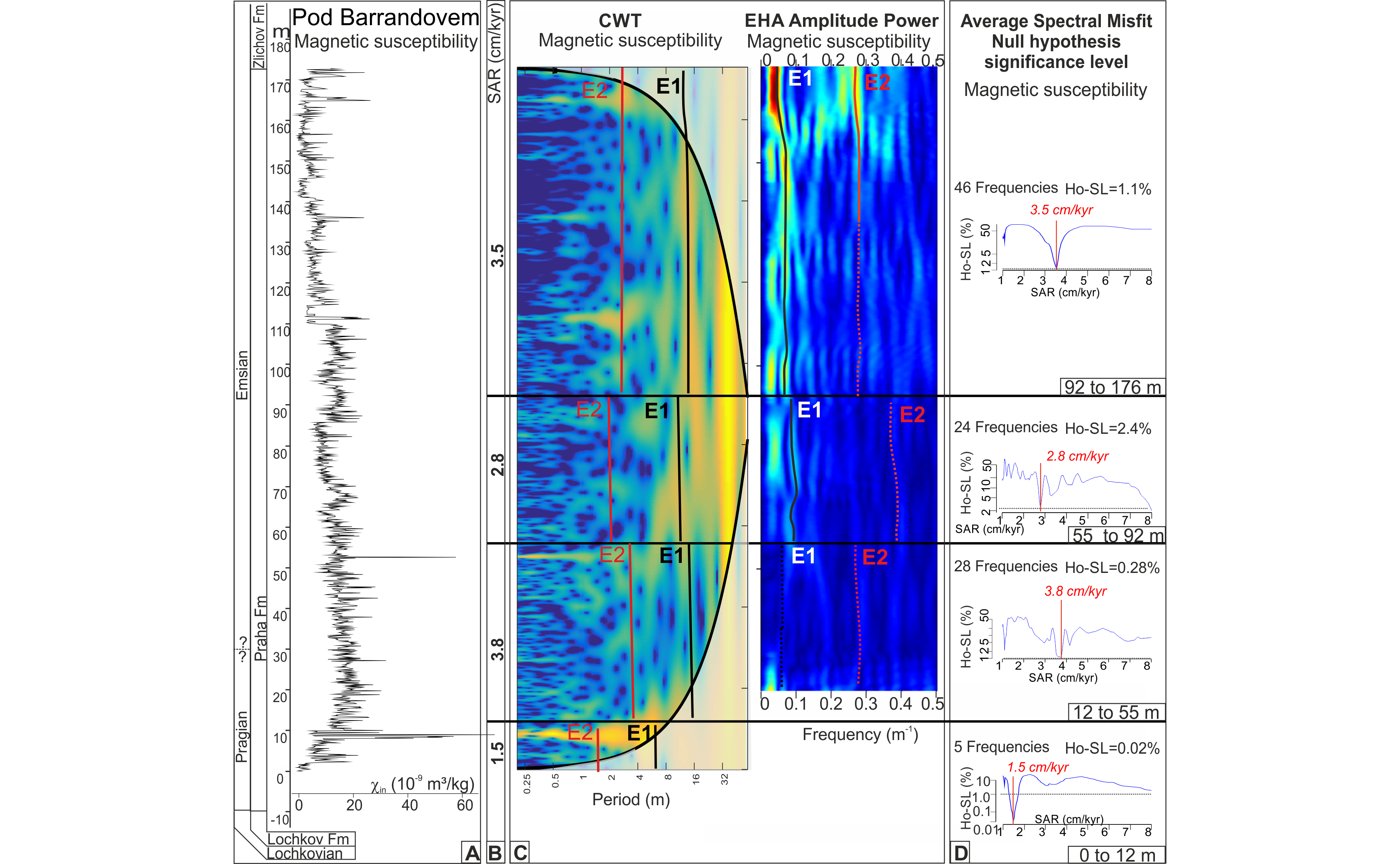
Figure 4. Pod Barrandovem section (Praha and Zlichov formations) with spectral analysis of the magnetic susceptibility (χin) record, reproduced from da Silva et al. (2016). The Zlichov Fm is not discussed in da Silva et al. (2016) and results are thus not shown. A. Stages of the geological time scale, rock formations and mass specific susceptibility record. B. Sediment accumulation rate (SAR) in cm/kyr, inferred from sedimentological, paleontological information, and assessment of the various spectral and statistical techniques: Continuous Wavelet Transform (CWT, panel C), Evolutive Harmonic Analysis (EHA, panel C), and Average Spectral Misfit (ASM, panel D). C. Continuous Wavelet Transform (CWT) and Evolutive Harmonic Analysis (EHA) of the susceptibility record. The interpreted 405 kyr eccentricity cycle (E1) and 100 kyr eccentricity cycle (E2) are shown with full lines when clear and with dotted lines when inferred. D. Average Spectral Misfit (ASM): the frequencies reaching 95% confidence level in the Multi-Taper-Taper Method (MTM) and related F-test (not shown here, see appendices in da Silva et al., 2016) are used as input for the ASM. The optimal SAR in cm/kyr from the ASM is given in red: it corresponds to the SAR with the lowest null hypothesis significance level (Ho_SL%). The number of input frequencies into the ASM obtained from MTM and F-test is also specified along with the optimal Ho_SL (%). Abbreviation: Fm, Formation.

77The study resulted in a much better constrained duration of the Praha Fm and the Pragian Stage: 5.7 ± 0.6 Myr and 1.7 ± 0.7 Myr respectively (da Silva et al., 2016), numbers that are included in the 2020 Geological Time Scale (Gradstein et al., 2020). Because of the rather long total duration in the study, including the Lochkovian Stage (7.7 ± 2.8 Myr), da Silva et al. (2016) find also strong indications for the long-period ~2.5 Myr and ~1 Myr eccentricity, and obliquity amplitude modulation cycles. The Praha Fm at Pod Barrandovem (and Pozar) consists of continuous deep pelagic suspension deposits, a deeper setting than the underlying Lochkov Fm which may be explanation for its well-developed spectral signatures.

78It is appropriate to finish here with a cautionary note. The Praha Fm extends well into the lower Emsian Stage. Yet, the directly overlying Zlichov Fm, Emsian as well, which was also sampled and subjected to the same set of analyses, does not enable a straightforward interpretation. At Pod Barrandovem both formations are on top of each other, only separated by a disturbed sediment bed. There may be a hiatus between the Praha and Zlichov formations but if present it is short because all conodont zones are present (Slavík, 2004). The Zlichov Fm is distinctly more clastic and chertier than the Praha Fm, so lithology is an important parameter to take into account.

4. Conclusions and perspectives

79Susceptibility is in principle a powerful proxy but a most meaningful interpretation of its variations requires that the underlying sources must be known. Is the variability in a record determined by the ferromagnetic contribution or the diamagnetic plus paramagnetic contribution? Extended rock magnetic characterization may include measurement of hysteresis loops to determine the high field slope representing diamagnetic plus paramagnetic contribution. The slope of the hysteresis loop at B = 0 is an approximation of the ferromagnetic contribution of the susceptibility. Direct measurement of the magnetic mineralogy may involve remanence measurements: anhysteretic remanent magnetization (ARM) or isothermal remanent magnetization (IRM) acquisition curves that provide information on the magnetic grain size and magnetic mineralogy. ARM tends to ‘over-expose’ (partially oxidized) magnetite because magnetite acquires a high ARM comparison to other magnetic minerals. This applies in particular to SD magnetite. Measuring temperature dependence of magnetization or susceptibility is also informative. Susceptibility vs temperature curves tend to overestimate the expression of magnetite because of its high susceptibility in comparison to other magnetic minerals. Measuring frequency dependence of susceptibility, an easy measurement with commonly available instruments, provides important information on ultrafine SP particles.

80In loess-paleosol sequences susceptibility records provide important paleoclimate information. Assessing the relevance of partially oxidized magnetite rims requires susceptibility measurement before and after annealing at 150 °C (see van Velzen & Dekkers, 1999), something that is not regularly done. Oxidation that occurred in situ and in the loess provenance area may be distinguished by assessing differences in loess and paleosol portions of a sequence. By measuring the susceptibility frequency dependence in several intervals (Schneider et al., 2025) the importance of pedogenesis can be assessed in much more detail.

81Traces of secondary formed ferrimagnetic minerals, i.e. magnetite, greigite, or pyrrhotite, may interfere with a depositional interpretation of a low-field susceptibility record. Effects play up particularly in sediments that typically have only weak signals. Effects of diagenesis and very low grade metamorphism can mask an original depositional signal but this is not occurring in every section. An original depositional signal may even be enhanced if a direct association of the secondary mineral with acknowledged clastic minerals can be demonstrated, for example, a direct magnetite-illite association where both are formed at the expense of original smectite. In remagnetized sections this must be tested for in each case study. In (partially) remagnetized sections measurement of the high-field susceptibility, the high field slope in hysteresis loops, bypasses issues of potential bias in low-field susceptibility records, as it is determined by the non-magnetic matrix minerals that reflect clastic input. An example exploiting the high-field susceptibility is the study Rodionov et al. (2003) on middle Ordovician sediments with a difficult to interpret paleomagnetic record. An aspect that should be assessed is the extent of differential diagenesis in limestone marl sequences. As recommended by Li J. et al. (2018) variations in Sr content between marl and limestone intervals serve to recognize whether a diagenetic system is open or closed, and oxygen and carbon stable isotope systematics unveil potential remobilization and oxidation of organic matter as a driver of diagenesis. Integration with other proxies, for example, geochemistry, -ray records (corrected for U amounts as U may have been mobilized) is desirable to constrain the interpretation of a susceptibility record.

82If a susceptibility record reflects a primary signature it can be utilized for paleoclimate analysis and as a duration chronometer in high resolution time scale construction. Evidently sample density should be higher than the Nyquist frequency of the shortest target cycle. For example, people recommend 4 to 6 samples per shortest target cycle. Also records should be sufficiently long for meaningful detection of low frequency cycles. Establishment of the long eccentricity cycle may become tedious in records shorter than ~1 Myr. Long period combination cycles thus require long records for a meaningful detection. Blindfold use of significance levels should be avoided, visual cyclicity should support any statistical inference. Susceptibility proxy records of sufficient resolution tap a substantial reservoir of information if the underlying drivers of its variability are well understood.

Acknowledgments

83The author thanks the Board of Geologica Belgica Luxemburga Scientia & Professionis for awarding him the André Dumont medal, and the editors of Geologica Belgica for their invitation to provide this paper. Geological Belgica reviewers Xavier Devleeschouwer and Leonardo Sagnotti are thanked for detailed input which was very helpful in fine-tuning this review.

References

84Aben, F.M., Dekkers, M.J., Bakker, R.R., van Hinsbergen, D.J.J., Zachariasse, W.J., Tate, G.W., McQuarrie, N., Harris, R. & Duffy, B., 2014. Untangling inconsistent magnetic polarity records through an integrated rock magnetic analysis: A case study on Neogene sections in East Timor. Geochemistry, Geophysics, Geosystems, 15, 2531–2554. https://doi.org/10.1002/2014GC005294

85Ahmed, I.A.M. & Maher, B.A., 2018. Identification and paleoclimatic significance of magnetite nanoparticles in soils. Proceedings of the National Academy of Sciences, 115, 1736–1741. https://doi.org/10.1073/pnas.1719186115

86An, Z., Kukla, G.J., Porter, S.C. & Xiao, J., 1991. Magnetic susceptibility evidence of monsoon variation on the Loess Plateau of central China during the last 130,000 years. Quaternary Research, 36, 29–36. https://doi.org/10.1016/0033-5894(91)90015-W

87Ao, H., Roberts, A.P., Dekkers, M.J., Liu, X., Rohling, E.J., Shi, Z., An, Z. & Zhao, X., 2016. Late Miocene–Pliocene Asian monsoon intensification linked to Antarctic ice-sheet growth. Earth and Planetary Science Letters, 444, 75–87. http://dx.doi.org/10.1016/j.epsl.2016.03.028

88Ao, H., Liebrand, D., Dekkers, M.J., Roberts, A.P., Jonell, T.N., Jin, Z., Song, Y., Liu, Q., Sun, Q., Li, X., Huang, C., Qiang, X. & Zhang, P., 2024. Orbital- and millennial-scale Asian winter monsoon variability across the Pliocene–Pleistocene glacial intensification. Nature Communications, 15, 3364. https://doi.org/10.1038/s41467-024-47274-9

89Aubourg, C., Pozzi, J.-P. & Kars, M., 2012. Burial, claystones remagnetization and some consequences for magnetostratigraphy. In Elmore, R.D., Muxworthy, A.R., Aldana, M.M. & Mena, M. (eds), Remagnetization and Chemical Alteration of Sedimentary Rocks. Geological Society, London, Special Publications, 371, 181–188. http://dx.doi.org/10.1144/SP371.4

90Aubourg, C., Jackson, M., Ducoux, M. & Mansour, M., 2019. Magnetite‐out and pyrrhotite‐in temperatures in shales and slates. Terra Nova, 31, 534–539. https://doi.org/10.1111/ter.12424

91Balsam, W.L., Ellwood, B.B., Ji, J., Williams, E.R., Long, X. & El Hassani, A., 2011. Magnetic susceptibility as a proxy for rainfall: Worldwide data from tropical and temperate climate. Quaternary Science Reviews, 30, 2732–2744. https://doi.org/10.1016/j.quascirev.2011.06.002

92Banerjee, S., Elmore, R.D. & Engel, M.H., 1997. Chemical remagnetization and burial diagenesis: testing the hypothesis in the Pennsylvanian Belden Formation, Colorado. Journal of Geophysical Research: Solid Earth, 102(B11), 24825–24842. https://doi.org/10.1029/97JB01893

93Begét, J.E. & Hawkins, D.B., 1989. Influence of orbital parameters on Pleistocene loess deposition in central Alaska. Nature, 337, 151–153. https://doi.org/10.1038/337151a0

94Berger, A., Loutre, M.F. & Laskar, J., 1992. Stability of astronomical frequencies over the Earth’s history for paleoclimate studies. Science, 255, 560–566. https://doi.org/10.1126/science.255.5044.560

95Bidegain, J.C., Evans, M.E. & van Velzen, A.J., 2005. A magnetoclimatological investigation of Pampean loess, Argentina. Geophysical Journal International, 160, 55–62. https://doi.org/10.1111/j.1365-246X.2004.02431.x

96Blakemore, R., 1975. Magnetotactic bacteria. Science, 190, 377–379. https://doi.org/10.1126/science.170679

97Borradaile, G.J. & Henry, B., 1997. Tectonic applications of magnetic susceptibility and its anisotropy. Earth-Science Reviews, 42, 49–93. https://doi.org/10.1016/S0012-8252(96)00044-X

98Borradaile, G.J. & Werner, T., 1994. Magnetic anisotropy of some phyllosilicates. Tectonophysics, 235, 223–248. https://doi.org/10.1016/0040-1951(94)90196-1

99Boulila, S., Galbrun, B., Miller, K.G., Pekar, S.F., Browning, J.V., Laskar, J. & Wright, J.D., 2011. On the origin of Cenozoic and Mesozoic “third-order” eustatic sequences. Earth-Science Reviews, 109, 94–112. https://doi.org/10.1016/j.earscirev.2011.09.003

100Bradák, B., Seto, Y., Stevens, T., Újvári, G., Fehér, K. & Költringer, C., 2021. Magnetic susceptibility in the European Loess Belt: New and existing models of magnetic enhancement in loess. Palaeogeography., Palaeoclimatology, Palaeoecology, 569, 110329. https://doi.org/10.1016/j.palaeo.2021.110329

101Burgardt, P. & Seehra, M.S., 1977. Magnetic susceptibility of iron pyrite (FeS₂) between 4.2 and 620 K. Solid State Communications, 22, 153–156. https://doi.org/10.1016/0038-1098(77)90422-7

102Chang, S.-B.R. & Kirschvink, J.L., 1989. Magnetofossils, the magnetization of the sediments, and the evolution of magnetite biomineralization. Annual Review of Earth & Planetary Sciences, 17, 169–195. https://doi.org/10.1146/annurev.ea.17.050189.001125

103Cifelli, F., Mattei, M., Hirt, A.M. & Günther, D., 2004. The origin of tectonic fabrics in ‘‘undeformed’’ clays: The early stages of deformation in extensional sedimentary basins. Geophysical Research Letters, 31, L09604. https://doi.org/10.1029/2004GL019609

104Crick, R.E., Ellwood, B.B., Hladil, J., El Hassani, A., Hrouda, F. & Chlupác, I., 2001. Magnetostratigraphy susceptibility of the Přídolian–Lochkovian (Silurian–Devonian) GSSP (Klonk, Czech Republic) and a coeval sequence in Anti-Atlas Morocco. Palaeogeography Palaeoclimatology, Palaeoecology, 167, 73–100. https://doi.org/10.1016/S0031-0182(00)00233-9

105Crouzet, C., Rochette, P. & Ménard, G., 2001. Experimental evaluation of thermal recording of successive polarities during uplift of metasediments. Geophysical Journal International, 145, 771–785. https://doi.org/10.1046/j.0956-540x.2001.01423.x

106Cui, Z., Liu, Q. & Etsell, T.H., 2002. Magnetic properties of ilmenite, hematite and oilsand minerals after roasting. Minerals Engineering, 15, 1121–1129. https://doi.org/10.1016/S0892-6875(02)00260-1

107Cullity, B.D. & Graham C.D., 2008. Introduction to Magnetic Materials. 2nd ed. Wiley, Hoboken (NJ), 544 p. https://doi.org/10.1002/9780470386323

108da Silva, A.-C., Hladil, J., Chadimová, L., Slavík, L., Hilgen, F.J., Bábek, O. & Dekkers, M.J., 2016. Refining the Early Devonian time scale using Milankovitch cyclicity in Lochkovian–Pragian sediments (Prague Synform, Czech Republic). Earth & Planetary Science Letters, 455, 125–139. https://doi.org/10.1016/j.epsl.2016.09.009

109Dearing, J.A., 1999. Magnetic susceptibility. In Walden J., Oldfield F. & Smith J. (eds.), Environmental magnetism: A practical guide. Quaternary Research Association, London, Technical Guide, 6, 35–62.

110Dearing, J.A., Dann, R.J.L., Hay, K., Lees, J.A., Loveland, P.J., Maher, B.A. & O’Grady, K., 1996. Frequency‐dependent susceptibility measurements of environmental materials. Geophysical Journal International, 124, 228–240. https://doi.org/10.1111/j.1365-246X.1996.tb06366.x

111Dinarès-Turell, J. & Dekkers, M.J., 1999. Diagenesis and remanence acquisition in the Lower Pliocene Trubi marls at Punta di Maiata (southern Sicily): palaeomagnetic and rock magnetic observations. In Tarling, D.H. & Turner, P. (eds), Palaeomagnetism and Diagenesis in Sediments. Geological Society, London, Special Publications, 151, 53–69. https://doi.org/10.1144/GSL.SP.1999.151.01.07

112Dunlop, D.J. & Özdemir, Ö., 1997. Rock Magnetism: Fundamentals and Frontiers. Cambridge University Press, Cambridge, 573 p. https://doi.org/10.1017/CBO9780511612794

113Egli, R., 2004. Characterization of individual rock magnetic components by analysis of remanence curves, 1. Unmixing natural sediments. Studia Geophysica Geodaetica, 48, 391–446. https://doi.org/10.1023/B:SGEG.0000020839.45304.6d

114Egli, R., 2009. Magnetic susceptibility measurements as a function of temperature and frequency I: Inversion theory. Geophysical Journal International, 177, 395–420. https://doi.org/10.1111/j.1365-246X.2009.04081.x

115Ellwood, B.B., Crick, R.E., El Hassani, A., Benoist, S.L. & Young, R.H., 2000. Magnetosusceptibility event and cyclostratigraphy method applied to marine rocks: Detrital input versus carbonate productivity. Geology, 28, 1135–1138. https://doi.org/10.1130/0091-7613(2000)28<1135:MEACMA>2.0.CO;2

116Elmore, R.D., Foucher, J.L.E., Evans, M., Lewchuk, M. & Cox, E., 2006. Remagnetization of the Tonoloway Formation and the Helderberg Group in the Central Appalachians: testing the origin of syntilting magnetizations. Geophysical Journal International, 166, 1062–1076. https://doi.org/10.1111/j.1365-246X.2006.02875.x

117Evans, M.E., 2001. Magnetoclimatology of aeolian sediments. Geophysical Journal International, 144, 495–497. https://doi.org/10.1046/j.0956-540X.2000.01317.x

118Evans, M.E. & Heller, F., 1994. Magnetic enhancement and palaeoclimate: study of a loess/palaeosol couplet across the Loess Plateau of China. Geophysical Journal International, 117, 257–264. https://doi.org/10.1111/j.1365-246X.1994.tb03316.x

119Fairbridge, R.W., 1967. Phases of diagenesis and authigenesis. In Larsen, G. & Chilingar, G.V. (eds), Diagenesis in Sediments. Elsevier, Amsterdam, Developments in Sedimentology, 8, 19–89. https://doi.org/10.1016/S0070-4571(08)70841-0

120Farina, M., Esquivel, D.M.S. & Lins de Barros, H.G.P., 1990. Magnetic iron-sulphur crystals from a magnetotactic microorganism. Nature, 343, 256–258. https://doi.org/10.1038/343256a0

121Fassbinder, J.W.E., Stanjek, H. & Vali, H., 1990. Occurrence of magnetic bacteria in soil. Nature, 343, 161–163. https://doi.org/10.1038/343161a0

122Forster, T., Evans, M.E. & Heller, F., 1994. The frequency dependence of low field susceptibility in loess sediments. Geophysical Journal International, 118, 636–642. https://doi.org/10.1111/j.1365-246X.1994.tb03990.x

123Gallo, L.C., Domeier, M., Antonio, P.Y., Sapienza, F., Rapalini, A., Font, E., Adatte, T., Trindade, R.I.F., Temporim, F., Tonti-Filippini, J., Silkoset, P. & Warre, L., 2025. Unraveling remagnetization sources using statistical learning. Earth & Planetary Science Letters, 662, 119390. https://doi.org/10.1016/j.epsl.2025.119390

124Geiss, C.E., Egli, R. & Zanner, C.W., 2008. Direct estimates of pedogenic magnetite as a tool to reconstruct past climates from buried soils. Journal of Geophysical Research: Solid Earth, 113, B11102. https://doi.org/10.1029/2008JB005669

125Grabowski, J., Bábek, O., Nawrocki, J. & Tomek, Č., 2008. New palaeomagnetic data from the Palaeozoic carbonates of the Moravo-Silesian Zone (Czech Republic): evidence for a timing and origin of the late Variscan remagnetization. Geological Quarterly, 52, 321–334. https://gq.pgi.gov.pl/article/view/7496/6146

126Gradstein, F.M., Ogg, J.G., Schmitz, M.D. & Ogg, G.M. (eds), 2020. Geologic Time Scale 2020. 2 vols. Elsevier, Amsterdam, 1357 p. https://doi.org/10.1016/C2020-1-02369-3

127Hällberg, L.P., Stevens, T., Almqvist, B., Snowball, I., Wiers, S., Költringer, C., Lu, H., Zhang, H. & Lin, Z., 2020. Magnetic susceptibility parameters as proxies for desert sediment provenance. Aeolian Research, 46, 100615. https://doi.org/10.1016/j.aeolia.2020.100615

128Harrison, R.J., Dunin-Borkowski, R.E. & Putnis, A., 2002. Direct imaging of nanoscale magnetic interactions in minerals. Proceedings of the National Academy of Sciences, 99, 16556–16561. https://doi.org/10.1073/pnas.262514499

129Heller, F. & Liu, T.S., 1982. Magnetostratigraphical dating of loess deposits in China. Nature, 300, 431–433. https://doi.org/10.1038/300431a0

130Heller, F., Shen, C.D., Beer, J., Liu, X.M., Liu, T.S., Bronger, A., Suter, M. & Bonani, G., 1993. Quantitative estimates of pedogenic ferromagnetic mineral formation in Chinese loess and palaeoclimatic implications. Earth & Planetary Science Letters, 114, 385–390. https://doi.org/10.1016/0012-821X(93)90038-B

131Hrouda, F., 2011. Models of frequency‐dependent susceptibility of rocks and soils revisited and broadened. Geophysical Journal International, 187, 1259–1269. https://doi.org/10.1111/j.1365-246X.2011.05227.x

132Hrouda, F., Chlupáčová, M. & Mrázová, S., 2006. Low-field variation of magnetic susceptibility as a tool for magnetic mineralogy of rocks. Physics of the Earth & Planetary Interiors, 154, 323–336. https://doi.org/10.1016/j.pepi.2005.09.013

133Hrouda, F., Pokorný, J., Ježek, J. & Chadima, M., 2013. Out‐of‐phase magnetic susceptibility of rocks and soils: A rapid tool for magnetic granulometry. Geophysical Journal International, 194, 170–181. https://doi.org/10.1093/gji/ggt097

134Huang, W., van Hinsbergen, D.J.J., Dekkers, M.J., Garzanti, E., Dupont-Nivet, G., Lippert, P.C., Li, X., Maffione, M., Langereis, C.G., Hu, X., Guo, Z. & Kapp, P., 2015. Paleolatitudes of the Tibetan Himalaya from primary and secondary magnetizations of Jurassic to Lower Cretaceous sedimentary rocks. Geochemistry, Geophysics, Geosystems, 16, 77–100. https://doi.org/10.1002/2014GC005624

135Hunt, C.P., Moskowitz, B.M. & Banerjee, S.K., 1995. Magnetic properties of rocks and minerals. In Ahrens, T.J. (ed.), Rock Physics and Phase Relations: Handbook of Physical Constants. American Geophysical Union, Washington DC, 189–204. https://doi.org/10.1029/RF003p0189

136Hüsing, S.K., Kuiper, K.F., Link, W., Hilgen, F.J. & Krijgsman, W., 2009. The upper Tortonian–lower Messinian at Monte dei Corvi (Northern Apennines, Italy): completing a Mediterranean reference section for the Tortonian Stage. Earth & Planetary Science Letters, 282, 140–157. https://doi.org/10.1016/j.epsl.2009.03.010

137Jackson, M. & Swanson-Hysell, N.L., 2012. Rock magnetism of remagnetized carbonate rocks: another look. In Elmore, R.D., Muxworthy, A.R., Aldana, M.M. & Mena, M. (eds), Remagnetization and Chemical Alteration of Sedimentary Rocks. Geological Society, London, Special Publications, 371, 229–251. https://doi.org/10.1144/SP371.3

138Jerolmack, D.J. & Paola, C., 2010. Shredding of environmental signals by sediment transport. Geophysical Research Letters, 37, L19401. http://dx.doi.org/10.1029/2010GL044638

139Jonsson, T., Mattsson, J., Nordblad, P. & Svedlindh, P., 1997. Energy barrier distribution of a noninteracting nano‐sized magnetic particle system. Journal of Magnetism & Magnetic Materials, 168, 269–277. https://doi.org/10.1016/S0304-8853(96)00710-X

140Just, J., Dekkers, M.J., von Dobeneck, T., van Hoesel, A. & Bickert, T., 2012. Signatures and significance of aeolian, fluvial, bacterial and diagenetic magnetic mineral fractions in Late Quaternary marine sediments off Gambia, NW Africa. Geochemistry, Geophysics, Geosystems, 13, Q0AO02. https://doi.org/10.1029/2012GC004146

141Kao, S.J., Horng, C.-S., Roberts, A.P. & Liu, K.K., 2004. Carbon–sulfur–iron relationships in sedimentary rocks from southwestern Taiwan: influence of geochemical environment on greigite and pyrrhotite formation. Chemical Geology, 203, 153–168. https://doi.org/10.1016/j.chemgeo.2003.09.007

142Kars, M., Aubourg, C., Labaume, P., Berquó, T.S. & Cavailhes, T., 2014. Burial diagenesis of magnetic minerals: New insights from the Grès d’Annot transect (SE France). Minerals, 4, 667–689. https://doi.org/10.3390/min4030667

143Katz, B., Elmore, R.D., Cogoini, M., Engel, M.H. & Ferry, S., 2000. Associations between burial diagenesis of smectite, chemical remagnetization, and magnetite authigenesis in the Vocontian trough, SE France. Journal of Geophysical Research: Solid Earth, B105, 851–868. https://doi.org/10.1029/1999JB900309

144Kelder, N.A., Sant, K., Dekkers, M.J., Magyar, I., van Dijk, G.A., Lathouwers, Y.Z., Sztanó, O. & Krijgsman, W., 2018. Paleomagnetism in Lake Pannon: Problems, pitfalls, and progress in using iron sulfides for magnetostratigraphy. Geochemistry, Geophysics, Geosystems, 19, 3405–3429. https://doi.org/10.1029/2018GC007673

145Kent, D.V., Olsen, P.E., Rasmussen, C., Lepre, C., Mundil, R., Irmis, R.B., Gehrels, G.E., Giesler, D., Geissman, J.W. & Parker, W.G., 2018. Empirical evidence for stability of the 405-kiloyear Jupiter–Venus eccentricity cycle over hundreds of millions of years. Proceedings of the National Academy of Sciences, 115, 6153–6158. https://doi.org/10.1073/pnas.1800891115

146Kirschvink, J.L. & Chang, S.-B.R., 1984. Ultrafine-grained magnetite in deep-sea sediments: Possible bacterial magnetofossils. Geology, 12, 559–562. https://doi.org/10.1130/0091-7613(1984)12<559:UMIDSP>2.0.CO;2

147Kopp, R.E. & Kirschvink, J.L., 2008. The identification and biogeochemical interpretation of fossil magnetotactic bacteria. Earth-Science Reviews, 86, 42–61. https://doi.org/10.1016/j.earscirev.2007.08.001

148Kravchinsky, V.A., Zykina, V.S., Zykin, V.S., 2008. Magnetic indicator of global paleoclimate cycles in Siberian loess–paleosol sequences. Earth & Planetary Science Letters, 265, 498–514. https://doi.org/10.1016/j.epsl.2007.10.031

149Krs, M., Pruner, P. & Man, O., 2001. Tectonic and paleogeographic interpretation of the paleomagnetism of Variscan and pre-Variscan formations of the Bohemian Massif, with special reference to the Barrandian terrane. Tectonophysics, 332, 93–114. https://doi.org/10.1016/S0040-1951(00)00251-1

150Kruiver, P.P., Dekkers, M.J. & Heslop, D., 2001. Quantification of magnetic coercivity components by the analysis of acquisition curves of isothermal remanent magnetisation. Earth & Planetary Science Letters, 189, 269–276. https://doi.org/10.1016/S0012-821X(01)00367-3

151Lantink, M.L., Davies, J.H.F.L., Ovtcharova, M. & Hilgen, F.J., 2022. Milankovitch cycles in banded iron formations constrain the Earth–Moon system 2.46 billion years ago. Proceedings of the National Academy of Sciences, 119, e2117146119. https://doi.org/10.1073/pnas.2117146119

152Larrasoaña, J.C., Roberts, A.P., Stoner, J.S., Richter, C. & Wehausen, R., 2003. A new proxy for bottom-water ventilation in the eastern Mediterranean based on diagenetically controlled magnetic properties of sapropel-bearing sediments. Palaeogeography, Palaeoclimatology, Palaeoecology, 190, 221–242. https://doi.org/10.1016/S0031-0182(02)00607-7

153Larrasoaña, J.C., Roberts, A.P., Musgrave, R.J., Gràcia, E., Piñero, E., Vega, M. & Martínez-Ruiz, F., 2007. Diagenetic formation of greigite and pyrrhotite in gas hydrate marine sedimentary systems. Earth & Planetary Science Letters, 261, 350–366. https://doi.org/10.1016/j.epsl.2007.06.032

154Laskar, J., Robutel, P., Joutel, F., Gastineau, M., Correia, A.C.M. & Levrard, B., 2004. A long-term numerical solution for the insolation quantities of the Earth. Astronomy & Astrophysics, 428, 261–285. https://doi.org/10.1051/0004-6361:20041335

155Laskar, J., Fienga, A., Gastineau, M. & Manche, H., 2011. La2010: a new orbital solution for the long-term motion of the Earth. Astronomy & Astrophysics, 532, A89. https://doi.org/10.1051/0004-6361/201116836

156Li, J., Cai, Z., Chen, H., Cong, F., Wang, L., Wei, Q. & Luo, Y., 2018. Influence of differential diagenesis on primary depositional signals in limestone-marl alternations: An example from Middle Permian marine successions, South China. Palaeogeography, Palaeoclimatology, Palaeoecology, 495, 139–151. https://doi.org/10.1016/j.palaeo.2018.01.002

157Li, J., Yamazaki, T., Usui, Y., Sagawa, T., Kubota, Y. & Kuroda, J., 2022. Understanding the role of biogenic magnetite in geomagnetic paleointensity recording: Insights from Ontong Java Plateau sediments. Journal of Geophysical Research: Solid Earth, 127, e2022JB024387. https://doi.org/10.1029/2022jb024387

158Li, M., Kump, L.R., Hinnov, L.A. & Mann, M.E., 2018. Tracking variable sedimentation rates and astronomical forcing in Phanerozoic paleoclimate proxy series with evolutionary correlation coefficients and hypothesis testing. Earth & Planetary Science Letters, 501, 165–179. https://doi.org/10.1016/j.epsl.2018.08.041

159Li, M., Hinnov, L. & Kump, L., 2019. Acycle: Time-series analysis software for paleoclimate research and education. Computers & Geosciences, 127, 12–22. https://doi.org/10.1016/j.cageo.2019.02.011

160Lowrie, W., 1990. Identification of ferromagnetic minerals in a rock by coercivity and unblocking temperature properties. Geophysical Research Letters, 17, 159–162. https://doi.org/10.1029/GL017i002p00159

161Lu, G., Marshak, S. & Kent D.V., 1990. Characteristics of magnetic carriers responsible for Late Paleozoic remagnetization in carbonate strata of the mid-continent, U.S.A. Earth & Planetary Science Letters, 99, 351–361. https://doi.org/10.1016/0012-821X(90)90139-O

162Maher, B.A., 2007. Environmental magnetism and climate change. Contemporary Physics, 48, 247–274. https://doi.org/10.1080/00107510801889726

163Maher, B.A., 2011. The magnetic properties of Quaternary aeolian dusts and sediments, and their palaeoclimatic significance. Aeolian Research, 3, 87–144. https://doi.org/10.1016/j.aeolia.2011.01.005

164Maher, B.A., 2016. Palaeoclimatic records of the loess/palaeosol sequences of the Chinese Loess Plateau. Quaternary Science Reviews, 154, 23–84. https://doi.org/10.1016/j.quascirev.2016.08.004

165Maher, B.A. & Thompson, R., 1995. Paleorainfall reconstructions from pedogenic magnetic susceptibility variations in the Chinese loess and paleosols. Quaternary Research, 44, 383–391. https://doi.org/10.1006/qres.1995.1083

166Maher, B.A., Thompson, R. & Zhou, L.P., 1994. Spatial and temporal reconstructions of changes in the Asian palaeomonsoon: a new mineral magnetic approach. Earth & Planetary Science Letters, 125, 461–471. https://doi.org/10.1016/0012-821X(94)90232-1

167Mann, S., Sparks, N.H.C., Frankel, R.B., Bazylinski, D.A. & Jannasch, H.W., 1990. Biomineralization of ferrimagnetic greigite (Fe₃S₄) and iron pyrite (FeS₂) in a magnetotactic bacterium. Nature, 343, 258–261. https://doi.org/10.1038/343258a0

168Martín-Hernández, F. & Hirt, A.M., 2003. The anisotropy of magnetic susceptibility in biotite, muscovite and chlorite single crystals. Tectonophysics, 367, 13–28. https://doi.org/10.1016/S0040-1951(03)00127-6

169Maxbauer, D.P., Feinberg, J.M. & Fox, D.L., 2016. MAX UnMix: A web application for unmixing magnetic coercivity distributions. Computers & Geosciences, 95, 140–145. https://doi.org/10.1016/j.cageo.2016.07.009

170McCabe, C. & Elmore, R.D., 1989. The occurrence and origin of Late Paleozoic remagnetization in the sedimentary rocks of North America. Reviews of Geophysics, 27, 471–494. https://doi.org/10.1029/RG027i004p00471

171McCabe, C., Van der Voo, R., Peacor, D.R., Scotese, C.R. & Freeman, R., 1983. Diagenetic magnetite carries ancient yet secondary remanence in some Paleozoic sedimentary carbonates. Geology, 11, 221–223. https://doi.org/10.1130/0091-7613(1983)11<221:DMCAYS>2.0.CO;2

172Meyers, S., 2021. Astrochron: a computational tool for astrochronology. Version 1.6. https://CRAN.R-project.org/package=astrochron.

173Mugiraneza, S. & Hallas, A.M., 2022. Tutorial: a beginner’s guide to interpreting magnetic susceptibility data with the Curie-Weiss law. Communcations Physics, 5, 95. https://doi.org/10.1038/s42005-022-00853-y

174Mullins, C.E. & Tite, M.S., 1973. Magnetic viscosity, quadrature susceptibility, and frequency dependence of susceptibility in single-domain assemblies of magnetite and maghemite. Journal of Geophysical Research, 78, 804–809. https://doi.org/10.1029/JB078i005p00804

175Néel, L., 1949. Théorie du traînage magnétique des ferromagnétiques en grains fins avec application aux terres cuites. Annales de Géophysique, 5, 99–136.

176Oliva-Urcia, B., Pueyo, E.L. & Larrasoaña, J.C., 2008. Magnetic reorientation induced by pressure solution: a potential mechanism for orogenic-scale remagnetizations. Earth & Planetary Science Letters, 265, 525–534. https://doi.org/10.1016/j.epsl.2007.10.032

177Oliver, J., 1986. Fluids expelled tectonically from orogenic belts: their role in hydrocarbon migration and other geologic phenomena. Geology, 14, 99–102. https://doi.org/10.1130/0091-7613(1986)14<99:FETFOB>2.0.CO;2

178Panaiotu, C.G., Panaiotu, E.C., Grama, A. & Necula, C., 2001. Paleoclimatic record from a loess-paleosol profile in Southeastern Romania. Physics and Chemistry of the Earth, Part A: Solid Earth and Geodesy, 26, 893–898. https://doi.org/10.1016/S1464-1895(01)00138-7

179Parés, J.M., 2015. Sixty years of anisotropy of magnetic susceptibility in deformed sedimentary rocks. Frontiers in Earth Science, 3, 4. https://doi.org/10.3389/feart.2015.00004

180Passier, H.F., de Lange, G.J. & Dekkers, M.J., 2001. Magnetic properties and geochemistry of the active oxidation front and the youngest sapropel in the eastern Mediterranean Sea. Geophysical Journal International, 145, 604–614. https://doi.org/10.1046/j.0956-540x.2001.01394.x

181Pastor-Galán, D., Groenewegen, T., Brouwer, D., Krijgsman, W. & Dekkers, M.J., 2015. One or two oroclines in the Variscan orogen of Iberia? Implications for Pangea amalgamation. Geology, 43, 527–530. https://dx.doi.org/10.1130/G36701.1

182Philo, J.S. & Fairbank, W.M., 1980. Temperature dependence of the diamagnetism of water. Journal of Chemical Physics, 72, 4429–4433. https://doi.org/10.1063/1.439734

183Rayleigh Lord, 1887. On the behaviour of iron and steel under the operation of feeble magnetic forces. Philosophical Magazine, 23(142), 225–245. https://doi.org/10.1080/14786448708628000

184Rickard, D., Roberts, A.P. & Navrotsky, A., 2024. Sedimentary greigite formation. American Journal of Science, 324, 13. https://doi.org/10.2475/001c.121855

185Roberts, A.P., 2015. Magnetic mineral diagenesis. Earth-Science Reviews, 151, 1–47. https://doi.org/10.1016/j.earscirev.2015.09.010

186Roberts, A.P., 2026. Mineral Magnetism. Cambridge University Press, Cambridge, 533 p. https://doi.org/10.1017/9781108935630

187Roberts, A.P. & Weaver, R., 2005. Multiple mechanisms of remagnetization involving sedimentary greigite (Fe₃S₄). Earth & Planetary Science Letters, 231, 263–277. https://doi.org/10.1016/j.epsl.2004.11.024

188Roberts, A.P., Chang, L., Rowan, C.J., Horng, C.-S. & Florindo, F., 2011. Magnetic properties of sedimentary greigite (Fe₃S₄): An update. Reviews of Geophysics, 49, RG1002. https://doi.org/10.1029/2010RG000336

189Roberts, A.P., Almeida, T.P., Church, N.S., Harrison, R.J., Heslop, D., Li, Y., Li, J., Muxworthy, A.R., Williams, W. & Zhao, X., 2017. Resolving the origin of pseudo-single domain magnetic behavior. Journal of Geophysical Research: Solid Earth, 122, 9534–9558. https://doi.org/10.1002/2017JB014860

190Rochette, P., 1987. Metamorphic control of the magnetic mineralogy of black shales in the Swiss Alps: toward the use of ‘magnetic isogrades’. Earth & Planetary Science Letters, 84, 446–456. https://doi.org/10.1016/0012-821X(87)90009-4

191Rochette, P. & Lamarche, G., 1986. Evolution des propriétés magnétiques lors des transformations minérales dans les roches : exemple du Jurassique Dauphinois (Alpes françaises). Bulletin de Minéralogie, 109, 687–696. https://doi.org/10.3406/bulmi.1986.7970

192Rochette, P., Jackson, M. & Aubourg, C., 1992. Rock magnetism and the interpretation of anisotropy of magnetic susceptibility. Reviews of Geophysics, 30, 209–226. https://doi.org/10.1029/92RG00733

193Rodionov, V.P., Dekkers, M.J., Khramov, A.N., Gurevich, E.L., Krijgsman, W., Duermeijer, C.E. & Heslop, D., 2003. Paleomagnetism and cyclostratigraphy of the Middle Ordovician Krivolutsky Suite, Krivaya Luka section, southern Siberian Platform: Record of non-synchronous NRM-components or a non-axial geomagnetic field? Studia Geophysica et Geodaetica, 47, 255–274. https://doi.org/10.1023/A:1023767523451

194Sagnotti, L., Cascella, A., Ciaranfi, N., Macrì, P., Maiorano, P., Marino, M. & Taddeucci, J., 2010. Rock magnetism and palaeomagnetism of the Montalbano Jonico section (Italy): Evidence for late diagenetic growth of greigite and implications for magnetostratigraphy. Geophysical Journal International, 180, 1049-1066. https://doi.org/10.1111/j.1365-246X.2009.04480.x

195Schill, E., Appel, E. & Gautam, P., 2002. Towards pyrrhotite/magnetite geothermometry in low-grade metamorphic carbonates of the Tethyan Himalayas (Shiar Khola, Central Nepal). Journal of Asian Earth Sciences, 20, 195–201. https://doi.org/10.1016/S1367-9120(01)00022-0

196Schmidt, V., Günther, D. & Hirt, A.M., 2006. Magnetic anisotropy of calcite at room-temperature. Tectonophysics, 418, 63–73. https://doi.org/10.1016/j.tecto.2005.12.019

197Schneider, R., Almqvist, B., Svedlindh, P., Hedlund, D., Thyr, J., Kurbanov, R. & Stevens, T., 2025. The more the merrier—Multi‐frequency magnetic susceptibility of loess and palaeosols as a sensitive climate proxy. Journal of Geophysical Research: Solid Earth, 130, e2024JB029727. https://doi.org/10.1029/2024JB029727

198Simmons, M.D., Miller, K.G., Ray, D.C, Davies, A., van Buchem, F.S.P. & Gréselle, B., 2020. Phanerozoic eustacy. In Gradstein, F.M., Ogg, J.G., Schmitz, M.D. & Ogg, G.M. (eds), Geologic Time Scale 2020. Elsevier, Amsterdam, 357–400. https://doi.org/10.1016/B978-0-12-824360-2.00013-9

199Slavík, L., 2004. The Pragian-Emsian conodont successions of the Barrandian area: search of an alternative to the GSSP polygnathid-based correlation concept. Geobios, 37, 454–470. https://doi.org/10.1016/j.geobios.2003.05.002

200Smith, D.G., 2023. The Orbital Cycle Factory: Sixty cyclostratigraphic spectra in need of re-evaluation. Palaeogeography, Palaeoclimatology, Palaeoecology, 628, 111744. https://doi.org/10.1016/j.palaeo.2023.111744

201Spassov, S., Heller, F., Kretzschmar, R., Evans, M.E., Yue, L.P. & Nourgaliev, D.K., 2003. Detrital and pedogenic magnetic mineral phases in the loess/palaeosol sequence at Lingtai (Central Chinese Loess Plateau). Physics of the Earth & Planetary Interiors, 140, 255–275. https://doi.org/10.1016/j.pepi.2003.09.003

202Spassov, S., Declercq, Y. & Egli, R., 2024. Exchange bias effect in Chinese loesses and palaeosols. Conference abstract. 18th New Trends on Paleo‐, Rock‐ and Environmental Magnetism meeting, Utrecht (The Netherlands).

203Suk, D.-W., Peacor, D.R. & Van der Voo, R., 1990a. Replacement of pyrite framboids by magnetite in limestone and implications for paleomagnetism. Nature, 345, 611–613. https://doi.org/10.1038/345611a0

204Suk, D.-W., Van der Voo, R. & Peacor, D.R., 1990b. Scanning and transmission electron microscope observations of magnetite and other iron phases in Ordovician carbonates from east Tennessee. Journal of Geophysical Research: Solid Earth, 95, 12327–12336. https://doi.org/10.1029/JB095iB08p12327

205Sun, D., Shaw, J., An, Z., Cheng, M. & Yue, L., 1998. Magnetostratigraphy and paleoclimatic interpretation of a continuous 7.2Ma Late Cenozoic eolian sediments from the Chinese Loess Plateau. Geophysical Research Letters, 25, 85–88. https://doi.org/10.1029/97GL03353

206Sun, Y., Clemens, S.C., An, Z. & Yu, Z., 2006. Astronomical timescale and palaeoclimatic implication of stacked 3.6-Myr monsoon records from the Chinese Loess Plateau. Quaternary Science Reviews, 25, 33–48. https://doi.org/10.1016/j.quascirev.2005.07.005

207Tarling, D.H. & Hrouda, F., 1993. The Magnetic Anisotropy of Rocks. Chapman & Hall, London, 217 p.

208Tauxe, L, Banerjee, S.K., Butler, R.F. & Van der Voo, R., 2018. Essentials of Paleomagnetism, 5th Web Edition. https://earthref.org/MagIC/books/Tauxe/Essentials/.

209Tohver, E., Weil, A.B., Solum, J.G. & Hall, C.M., 2008. Direct dating of carbonate remagnetization by ⁴⁰Ar/ ³⁹Ar analysis of the smectite–illite transformation. Earth & Planetary Science Letters, 274, 524–530. https://doi.org/10.1016/j.epsl.2008.08.002

210Újvári, G., Kok, J.F., Varga, G. & Kovács, J., 2016. The physics of wind-blown loess: implications for grain size proxy interpretations in Quaternary paleoclimate studies. Earth-Science Reviews, 154, 247–278. https://doi.org/10.1016/j.earscirev.2016.01.006

211Usui, Y., Yamazaki, T. & Saitoh, M., 2017. Changing abundance of magnetofossil morphologies in pelagic red clay around Minamitorishima, Western North Pacific. Geochemistry, Geophysics, Geosystems, 18, 4558–4572. https://doi.org/10.1002/2017gc007127

212Van der Voo, R. & Torsvik, T.H., 2012. The history of remagnetization of sedimentary rocks: deceptions, developments and discoveries. In Elmore, R.D., Muxworthy, A.R., Aldana, M.M. & Mena, M. (eds), Remagnetization and Chemical Alteration of Sedimentary Rocks. Geological Society, London, Special Publications, 371, 23–53. https://doi.org/10.1144/SP371.2

213Van Velzen, A.J. & Dekkers, M.J., 1999. Low-temperature oxidation of magnetite in loess-paleosol sequences: a correction of rock magnetic parameters. Studia Geophysica et Geodaetica, 43, 357–375. https://doi.org/10.1023/A:1023278901491

214Van Velzen, A.J. & Zijderveld, J.D.A., 1995. Effects of weathering on single-domain magnetite in Early Pliocene marine marls. Geophysical Journal International, 121, 267–278. https://doi.org/10.1111/j.1365-246X.1995.tb03526.x

215Vasiliev, I., Franke, C., Meeldijk, J.D., Dekkers, M.J., Langereis, C.G. & Krijgsman, W., 2008. Putative greigite magnetofossils from the Pliocene epoch. Nature Geoscience, 1, 782–786. https://doi.org/10.1038/ngeo335.

216Weaver, R., Roberts, A.P. & Barker, A.J., 2002. A late diagenetic (syn-folding) magnetization carried by pyrrhotite: implications for paleomagnetic studies from magnetic iron sulphide-bearing sediments. Earth & Planetary Science Letters, 200, 371–388. https://doi.org/10.1016/S0012-821X(02)00652-0

217Weedon, G.P., 2022. Problems with the current practice of spectral analysis in cyclostratigraphy: Avoiding false detection of regular cyclicity. Earth-Science Reviews, 235, 104261. https://doi.org/10.1016/j.earscirev.2022.104261

218Weil, A.B. & Van der Voo, R., 2002. Insights into the mechanism for orogen-related carbonate remagnetization from growth of authigenic Fe-oxide: A scanning electron microscopy and rock magnetic study of Devonian carbonates from northern Spain. Journal of Geophysical Research: Solid Earth, 107, EPM 1. https://doi.org/10.1029/2001JB000200

219Weil, A.B., Gutiérrez-Alonso, G. & Conan, J., 2010. New time constraints on lithospheric-scale oroclinal bending of the Ibero-Armorican Arc: A palaeomagnetic study of earliest Permian rocks from Iberia. Journal of the Geological Society, London, 167, 127–143. https://doi.org/10.1144/0016-76492009-002

220Yamazaki, T. & Ikehara, M., 2012. Origin of magnetic mineral concentration variation in the Southern Ocean. Paleoceanography, 27, PA2206. https://doi.org/10.1029/2011pa002271

221Zeeden, C., Kels, H., Hambach, U., Schulte, P., Protze, J., Eckmeier, E., Marković, S.B., Klasen, N. & Lehmkuhl, F., 2016. Three climatic cycles recorded in a loess-palaeosol sequence at Semlac (Romania) – Implications for dust accumulation in south-eastern Europe. Quaternary Science Reviews, 154, 130–142. https://doi.org/10.1016/j.quascirev.2016.11.002

222Zeeden, C., Hambach, U., Veres, D., Fitzsimmons, K., Obreht, I., Bösken, J. & Lehmkuhl, F., 2018. Millennial scale climate oscillations recorded in the Lower Danube loess over the last glacial period. Palaeogeography, Palaeoclimatology, Palaeoecology, 509, 164–181. https://doi.org/10.1016/j.palaeo.2016.12.029

223Zegers, T.E., Dekkers, M.J. & Bailly, S., 2003. Late Carboniferous to Permian remagnetization of Devonian limestones in the Ardennes: role of temperature, fluids, and deformation. Journal of Geophysical Research: Solid Earth, 108, 2357. https://doi.org/10.1029/2002JB002213

224Zwing, A., Matzka, J., Bachtadse, V. & Soffel, H.C., 2005. Rock magnetic properties of remagnetized Palaeozoic clastic and carbonate rocks from the NE Rhenish massif, Germany. Geophysical Journal International, 160, 477–486. https://doi.org/10.1111/j.1365-246X.2004.02493.x

225Manuscript received 18.11.2025, accepted in revised form 27.02.2026, available online 05.06.2026.

Para citar este artículo

Acerca de: Mark J. DEKKERS