Suzanne A.G. LEROY, Françoise CHALIÉ, Frank P. WESSELINGH, Mohammad Saeed SANJANI, Hamid A.K. LAHIJANI, John ATHERSUCH, Ulrich STRUCK, Gill PLUNKETT, Paula J. REIMER, Parisa HABIBI, Keivan KABIRI, Safiyeh HAGHANI, Abdolmajid NADERI BENI & Klaus ARPE

Multi-proxy indicators in a Pontocaspian system: a depth transect of surface sediment in the SE Caspian Sea

Document(s) associé(s)

Annexes

• GB 21-3-4 Leroy et al (8,3M)
• GB 21-3-4 Leroy et al_Supplem. Mat (2,0M)

Abstract

The response of large water-bodies to global change in terms of ecosystem services and economical value is a major concern. The Caspian Sea, the world’s largest enclosed water-body, has a poorly-known water-level history, but observed changes are a hundred times faster than recent global sea-level rise. This ancient lake, characterised by brackish waters, is rich in endemic species; some of them have spread to similar environments worldwide. However, the ecology of Pontocaspian species remains poorly understood and must be studied in their original habitat.

This work aims at improving the capacity to reconstruct Quaternary environments of the Pontocaspian region and to provide a benchmark for biodiversity turnover studies. A transect of surface sediment across a wide shelf was subjected to multidisciplinary analyses: stable isotopes, pollen, dinocysts, diatoms, foraminifers, ostracods and molluscs and vertical oceanographic profiles.

Three depositional environments with characteristic communities were found: shore face, shelf and slope. Invasion impact was strongly felt by the molluscs. All biota groups, except diatoms, reflected high endemism. The radiocarbon reservoir effect is highlighted in differential ¹⁴C ages for different groups. Understanding such discrepancies require detailed insight into reworking processes. Tephra presence in the sediment shows a potential for tephrochronology. Stable isotope ratios in ostracods appear to reflect temperature depth gradients. Our results provide a baseline for calibrating proxy data to the present Pontocaspian environment.

Table des matières

1. Introduction

1The lack of long-term data on the response of aquatic systems to water-level and climatic changes is seen as an impediment to the assessment of the vulnerability and risks that large water-bodies face with respect to ongoing and future global changes. Petroleum, fishing (e.g. for caviar) and tourism industries, and governments are struggling to understand the vulnerabilities and risk associated with the unprecedented rate of environmental change and the consequences for ecosystems and natural resources such as water upon which we closely depend (Zonn et al., 2010). The Caspian Sea is a closed water body between Europe and Asia (Fig. 1A), of ~371,000 km² in size. Its water-levels are changing a hundred times faster than that of global ocean. For example water levels dropped 3 m between 1929 and 1977 (~6.2 cm yr^-1), and rose 2.3 m between 1977 and 1995 (~12.1 cm yr^-1) (Arpe et al., 2000; Kroonenberg et al., 2007). The rise since 1978 has been shown to be due to changes in atmospheric circulation and is strongly influenced by the discharge of the Volga River (Arpe & Leroy, 2007). Much too often, economic activities around the Caspian Sea cannot adapt to these rapid changes. Caspian Sea level has varied by as much as 10 m over the past millennium (Naderi Beni et al., 2013), although this has been partly due to human impact (Haghani et al., 2016).

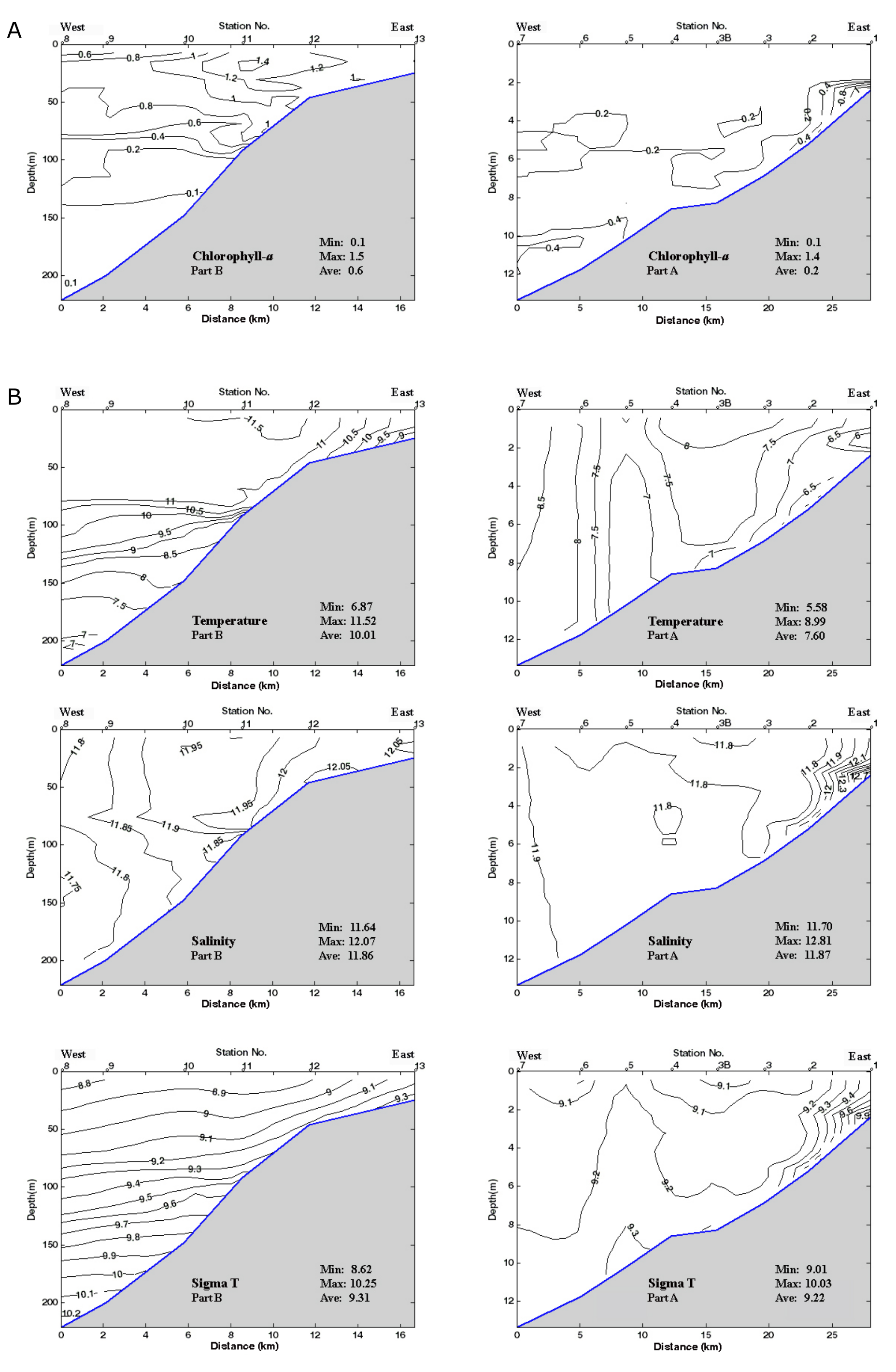
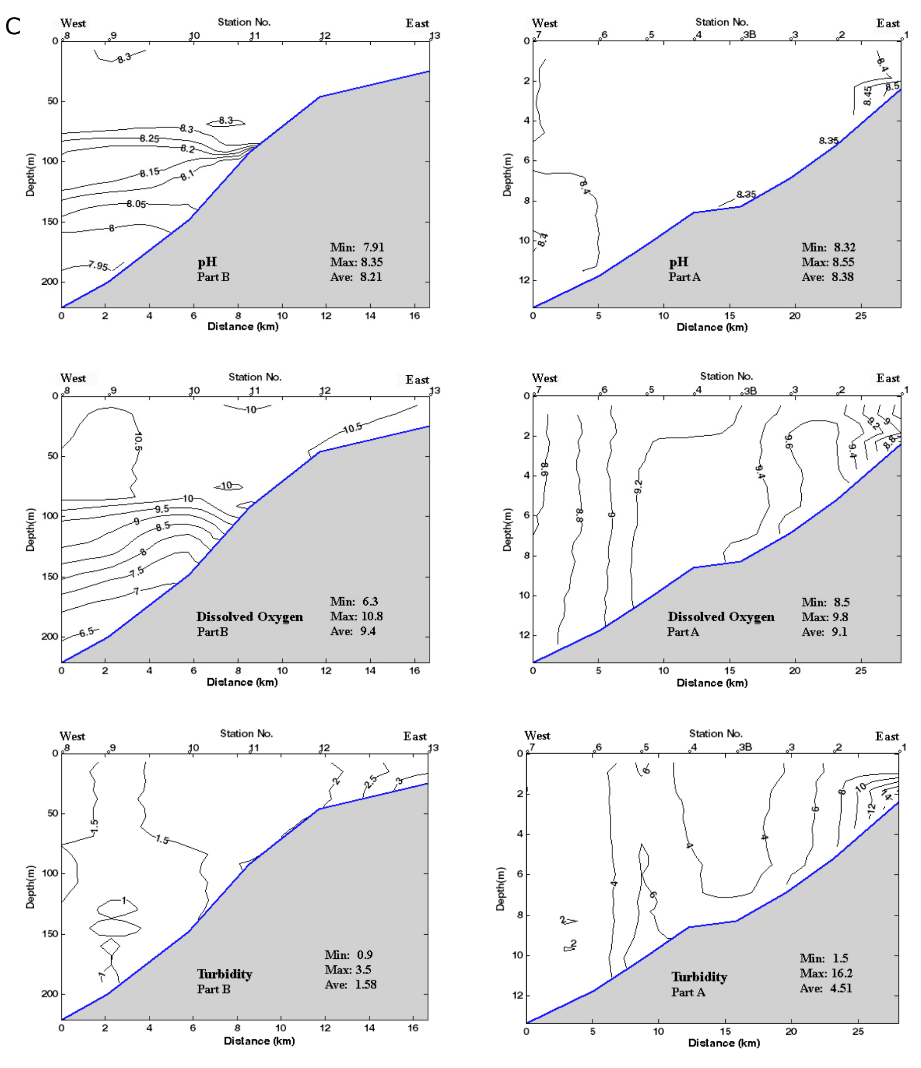
2Figure 1. Location. 1A: The Caspian Sea at the boundary between Europe and Asia with other Pontocaspian seas such as the Black and the Aral Sea. 1B: The southern basin of the Caspian Sea with the location of short cores referred to in the text. 1C: Location of the stations with their station number (upper number in italic) and their depths in m (lower number in bold) in two parts of the transect, A in the east and B in the west. See Table SI 1 for more information.

3It is essential to understand the mechanisms driving these changes; but so far, they have remained rather unclear. Very few of the Quaternary sedimentological and palaeontological tools used to reconstruct sea-level changes elsewhere in the world are suitable for the Caspian Sea (see why, later on in this paper). Hence it has become necessary to develop a more complex multi-proxy approach for reconstructing Caspian Sea levels. Some potential proxies for examining past water levels, salinities and temperatures in the Caspian Sea come from micro and macro-palaeontology: organic-walled dinoflagellate cysts, diatoms, foraminifers, ostracods and molluscs. However, its isolation from the world ocean ~2 Ma ago (Forte & Cowgill, 2013) has resulted in a very diverse, mostly endemic biota that makes the Caspian Sea an example of a long-lived biodiverse lake; but this biodiversity is threatened by recent invasions(Karpinsky, 2005a, 2005b). Only a limited number of modern calibration sets are available. A few collections of modern samples with measured physico-chemical parameters (such as water temperature, salinity, pH and nutrients) exist for any of those groups with the exception of the pioneering ostracod study by Gofman (1966), which has some limitations (see below). This greatly limits any quantitative reconstructions of past environments from biological data (Birks, 2003).

4We struggle to understand the history of the Caspian Sea due to i) endemism, ii) limited ecological range knowledge, iii) complex stable isotope drivers complicated by its isolated nature, iv) sediment dating difficulties, v) active tectonics affecting water-level reconstructions, vi) lack of research vessels, vii) confidentiality linked to data obtained by petroleum companies, viii) climatic models not taking in account the dynamic water levels, amongst other reasons. Therefore, the aims of the present study are to work towards establishing a new calibration set for the Caspian Sea in order to improve Quaternary environmental reconstructions. These could also be used elsewhere in the Pontocaspian region from the Black Sea to the Aral Sea, including some Anatolian lakes. Moreover, this type of multidisciplinary approach may serve as an example of what might be achieved in other parts of the world. This may be in: i) lakes with high endemism, e.g. Lake Ohrid, Lake Baikal and Lake Tanganyika (Albrecht & Wilke, 2008), which are in need of both detailed baseline studies (before conservation or restoration) and well-established calibration sets of endemic species for Quaternary investigations, and ii) bodies of brackish water originating from mixing of fresh and marine water in the historical or geological past, e.g. Baltic and White Seas (Karpinsky, 2005b). Moreover, to understand the behaviour of Pontocaspian invasive species worldwide (e.g. Dreissena polymorpha), it is first of all essential to understand it in the Pontocaspian area itself.

5The area chosen for this study is the south-east corner of the Caspian Sea (offshore Gorgan, SW Iran), as several palaeo-records have already been obtained in this region (e.g. Leroy et al., 2011, 2013a; Naderi Beni et al., 2013; Kakroodi et al., 2015) (Fig. 1B). The objectives of this study are to analyse a set of surface samples at the water–mud interface along a transect between water depths of 2 and 221 m using a wide range of techniques. Among the proxies applied some have proven to be useful in the Quaternary of the Caspian Sea and others are still in their infancy. The sedimentary composition was tackled using analysis of water, carbonate and organic matter content, particle size and magnetic susceptibility. The biological proxies consisted of pollen and spores recruited by wind and water to the site, planktonic forms such as dinocysts and most diatoms, and benthic forms comprising foraminifers, ostracods and molluscs. StableOand C isotopes were measured on the last three groups. The results are examined in relation to modern conditions, such as conductivity, temperature and depth data (CTD). In addition ¹⁴C dates were obtained and tephra occurrence tests were made.

2. Setting

2.1. The Caspian Sea and its surrounding

6The Caspian Sea is the world’s largest lake, both in terms of area and volume, extending 35–48ºN (>1000 km) and 47–55°E (Fig. 1A). Because of its great meridional extent, the Caspian Sea straddles several climatic zones. The south-western and the southern regions lie in a subtropical humid climatic zone; while the eastern coast has a desert climate. The study region shows a similar gradient from desertic along the coastal to subtropical humid on the northern foothills of the nearby Alborz Mountains (Fig. 1C).

7The Caspian Sea is located to the east of the Greater Caucasus and to the north of the Alborz Mountains, from which it is separated by a narrow stretch of lowland. Both mountain ranges are tectonically active and have featured volcanism during the Holocene (Karakhanian et al., 2003; Davidson et al., 2004). To the east, a series of arid plateaux separate the Caspian basin from the Turkmenistan deserts. The northern end of the basin is surrounded by the low-lying Caspian Depression.

8Many large rivers, notably the Volga, drain into the Caspian Sea, but no outlets exist; so water-levels (currently at 27 m below sea level (bsl)) are controlled by precipitation and evaporation over the water and its catchments (Kostianoy & Kosarev, 2005; Arpe & Leroy, 2007). Three basins divide the water body, becoming progressively deeper towards the south. The southern basin (168,000 km²) has an average depth of 325 m and a maximum depth of 1025 m. It holds more than 65% of the Caspian Sea water. The Apsheron sill (180 m water depth) divides the middle and southern basins.

9From a maximum in 1995 to the end of 2014, the Caspian Sea level decreased by 1.20 m (Arpe et al., 2014). Summer precipitation over the Volga basin is currently the main forcing factor (Arpe et al., 2012). The forecasting of water-level fluctuations is still being tested month by month (Arpe et al., 2014). Present salinities vary from less than 1 practical salinity unit (psu) in the Volga delta to 14 psu in summer offshore the desertic coast of Turkmenistan (Leroy et al., 2006; Matishov et al., 2012; Richards et al., 2014). An almost homogeneous 12.5–13.5 psu salinity is observed in the middle and southern basins. In the southern basin, seasonal salinity changes are <~0.2–0.4 psu. The mean annual salinity variation increases from the surface to the bottom waters from 0.1 to 0.3 psu (Zenkevitch, 1963; Kosarev & Yablonskaya, 1994; Peeters et al., 2000). The range of past surface salinities is not known but the southern and middle basins of the Caspian Sea might have fluctuated between 4 and 14 psu (low when the water level were high, and high during periods of low water levels) on the basis of estimations made from a comparison of the fossil organic-walled dinoflagellate cysts with the present-day in the Caspian Sea and with the Black Sea in the Early Holocene (Leroy et al., 2007, 2013a, 2013b, 2013c, 2014).

10The mean water-surface temperature in winter ranges from 0 ºC (when it is covered with ice) in the north to 10 ºC in the south, and in summer from 21 ºC in the west to 28 ºC in the south-east. A sharp thermocline occurs between 20 and 40 m during the summer, with almost negligible seasonal temperature fluctuations of the deeper waters (water temperatures ranges from 4.5 to 6 ºC below 200 m) (Zenkevitch, 1963). Deeper waters are well mixed. A clear water-surface temperature increase has been noted in the last few decades, especially for summer temperatures (Arpe et al., 2014; Leroy et al., 2013b).

2.2. Characteristics of the southern basin

11During winter, water-surface temperature in the coastal area of the southern basin (~7 ºC) is about half of that in the centre (~14 ºC) (Ibrayev et al., 2010). Along the east coast, two counter currents are superimposed: a northward surface and a southward deep current (Bondarenko, 1993; Kosarev & Yablonskaya, 1994; Ibrayev et al., 2010). The thickness of the water-mixing zone varies from 15–25 m in the west to 10 m towards the east coast of the southern Caspian Sea basin. Salinity of the surface water increases from west to east because of riverine input in the west and enhanced evaporation in the east. As for the whole Caspian Sea, vertical changes in salinity in the southern Caspian Sea basin are <1 psu. Therefore stratification depends more on the temperature gradient. Local sinking happens mainly in the eastern part due to evaporation and formation of saline dense water in the warm period, as well as evaporation and convective mixing in the colder months of the year. An upwelling of colder subsurface water along the east coast has been described for the middle basin (Ibrayev et al., 2010).

12Wind directions at a height of 10 m are predominantly from the North, turning slightly to Northwest with enhanced speeds in summer (Fig. SI 1 [Figures SI n and Tables SI n are available online as supplementary materials; see GB 21-3-4 Leroy et al._Supplem. Mat.pdf]; ECMWF, 2015). The winds (direction and speed) suggest possible upwelling only for autumn and winter along the east coast (Fig. SI 1). However the shallow bathymetry and the two superimposed counter currents prevent strong upwelling from developing in the east coast of the south basin. Wave heights may reach 3 m every year (Kouraev et al., 2011); so the calculated breaking depth is 3.8 m (Komar, 1998). This has implications for understanding the depth at which sediment may become mixed by wave action.

13The main characteristic of the bottom topography in the SE Caspian Sea basin is a gentle slope with a ~70 km wide shelf on the east coast. Two longshore currents, eastward on the south coast and southward on the east coast, meet each other (Lahijani et al., 2009). These horizontal movements have formed the Miankaleh Spit and the Gomishan Bay respectively (Fig. 1C). The sedimentation rate is thus very high in the area.

14The main river entering the SE area is the Gorgan River with a 12,000 km² drainage basin and a length of 350 km (Lahijani et al., 2008). It crosses the Kopet-Dagh Mountains (eastern extension of the Apsheron Sill, Fig.1A) and brings 3 million tonnes per year of fine sediment rich in carbonate to the Caspian Sea. The water discharge was around 0.4 km³ per year until recently (Lahijani et al., 2008); however since then, it has become ephemeral as it nearly stops flowing in summer. Its delta is river-dominated and it enters the Caspian Sea on a gently-sloping coast (nearshore and shelf). Artificial structures regulate its course upstream. Its strongest flow (still minor compared to other rivers in the south) is in spring, when it is fed by meltwater from the Alborz Mountains (Lahijani et al., 2008). Satellite pictures from Google Earth in 1984 show a plume reaching a maximum of 5 km westwards. Since then the plume size has dramatically decreased.

2.3. Biological setting

15The vegetation in the south-eastern corner of the Caspian Sea is dominated by Tamarix and by halophytes with Artemisia and Astragalus formations a few kilometres further inland around the Gorgan river course (Walter & Breckle, 1991). The southern coast lies within the Hyrcanian forest zone. Low altitudes are characterised by the Querco-Carpinetum plant formation that quickly changes with elevation on the northern slope of the Alborz Mountains into Parrotio-Carpinetum, Fagetum hyrcanum, and above 2000 m to Carpinetum orientalis/Quercus macranthera. The upper woody latitudinal zone above 2500 m consists of Juniperus excelsa (Walter & Breckle, 1991).

16Regarding the aquatic biology,the Caspian Sea is rich in endemic Caspian and Pontocaspian (shared only with the Black and the Aral Seas and some Turkish lakes) species. They have largely been naturally selected for their euryhalinity (Dumont, 1998). Due to the large number of endemics and to the paucity of morphological characteristics, the taxonomy of many groups is difficult and often confusing. For diatoms and ostracods, most of the reference literature concerning endemic species and the subtle description of morphology-based features supporting taxonomy is often written in Russian language, and so difficult to find and compile.

17It is remarkable that all the Caspian Sea foraminifers are benthic species. The extinction of planktonic taxa is likely linked to the recurrence of surface freshwater phases during the Quaternary (H. Oberhänsli, pers. commun. 2015). In the Caspian Sea, the depth limit for the occurrence of benthic foraminifers is poorly documented although it is often mentioned as being no more than 50 to 70 m water depth (Boomer et al., 2005; Yanko-Hombach, 2007; Kh. Saidova, pers. commun. 2011). A study of Caspian Sea sediments, between 1 and 840 m water-depth in the shallow northern basin and the deep water N and S of the Apsheron Peninsula (sill between the middle and south basins, Fig. 1A), shows that living foraminifers are not present below 60 m (Mayer, 1972). However it remains unclear why they are absent below this depth.

18All ostracods in the Caspian Sea are benthic. Gofman (1966) published in Russian the results of a detailed study on the distribution of ostracods from bottom samples collected from numerous locations across the Caspian Sea (with the notable exception of the Iranian sector). Her publication also includes detailed records of physical and chemical parameters at each site. This work was summarised and augmented in English by Yassini (1986). In addition, Boomer et al. (2005) recorded the depth distribution of ostracods from a number of locations.

19Distribution data for molluscs were presented by Kosarev & Yablonskaya (1994) in a comprehensive review, although it is based on an indirect relation to environmental parameters. Amongst others, the study clearly indicates that the abundance of invasive species is greatest in water <50 m. Below this depth, invasive species are rare or absent.

20The Caspian Sea has been subject to many biological invasions (Grigorovitch et al., 2003). A good example is that of the ctenophore Mnemiopsis leidyi in 1999 (Roohi & Sajjadi, 2011; Nasrollahzadeh et al., 2014). This comb jelly had a negative impact on zooplankton on which it feeds, triggering a phytoplankton biomass increase. Many studies of phytoplankton over the last twenty years focused on the southern basin of the Caspian Sea and relate recent phytoplankton composition fluctuations to human activities (Roohi et al., 2010; Bagheri et al., 2012; Tahami & Pourgholam, 2013; Gasanova et al., 2014). It is also noteworthy to indicate that many Pontocaspian species (e.g. Dreissena polymorpha) are invasive elsewhere in the world, e.g. the Baltic Sea, European inland waters and the Great lakes (Ojaveer et al., 2002).

3. Material and methods

21A transect of vertical oceanographic profiles and surface sediment was sampled on 9 and 10 February 2014 off-shore Gorgan, Iran, in the SE Caspian Sea. Sampling was performed in two parts: the first part (A) was in the easternmost section from the harbour of Bandar-e-Torkman and covered the shelf, and the second (B) comprised the western part of the transect from the harbour of Amirabad and includes the shelf break and part of the slope to greater depths (Fig. 1C;Table SI 1). When part A and part B are joined together, the transect is 81.4 km long, roughly parallel to the Gorgan Bay and starting close to the Gorgan River mouth. The sampling density of the stations has been a priori selected to reflect the areas with more or less potential changes.

3.1. Oceanography

22Oceanographic parameters were measured using a CTD “ocean seven 316” probe, developed by IDRONAUT (Italy), hosted at the Iranian National Institute of Oceanography and Atmospheric Sciences (INIOAS). After calibration of the sensors, the CTD probe was adjusted to collect data with a time interval of one second (Table SI 2). The CTD probe was released into the water column with a speed of 1 m/s from surface to bottom in all stations (except Station 8 where the probe was released to a depth of 221 m, 30 m above water bottom). Because of the closed nature of the Caspian Sea and the unique physical properties of its water, salinity and density (sigma-T) parameters had to be recalculated by applying a correction coefficient to the commonly used methodology from UNESCO (1983), which is only valid for standard sea water. Peeters et al. (2000) showed that the salinity computed from CTD data using the standard processes of UNESCO (1981) is systematically lower than the salinity recorded using chemical methods. The best agreement between the two methods was obtained by applying a correction factor (c_f) of 1.1017 as follows:

23S_casp = c_f × S_sea

24where S_sea is the salinity computed using the CTD cast and UNESCO equations, and S_casp is the corrected salinity for Caspian Sea water. For measuring in situ Chlorophyll-a (Chl-a), a Seapoint Chlorophyll Fluorometer (SCF) sensor was used.

25In addition, Chl-a values and SST were extracted from NASA MODIS-Aqua products for eight cloud-free days in 2013 and 2014 (two days of summer 2013, two days in winter 2013-2014, two days of summer 2014, and two days of winter 2014-2015). The remotely sensed Chl-a values (in units of mg m^-3) are determined using the OC3M algorithm, i.e. a fourth-order polynomial relationship between a ratio of R_rs (Remote sensing reflectance) and Chl-a values (Werdell & Bailey, 2005). On the other hand, SST values are determined based on the methodology developed by Minnett et al. (2004).

3.2. Sediment sampling

26Thirteen samples of ~500 g of wet sediment were taken from the top 1 cm of sediment (Table SI 1). It is not known how much time this represents, probably a few months or, at most, a few years. The time encapsulated in each the sample may vary along the transect. Grab samples along transect A were obtained from 2 to 13 m water depth from the side of an inflatable motor boat along the eastern part of the transect (Fig. 1C) and Kajak core tops (most of transect B) from 25 to 221 m water depth from the side of a fishing boat along the western part of the transect (Fig. 1C). In both cases, while still on board, the topmost 1 cm was carefully scooped out with a spoon in order to have the most recent sediment only. If necessary several grabs or core tops were taken in each station until a sufficient amount of sediment was obtained.

3.3. Sedimentology

27Particle size, loss-on-ignition (LOI), magnetic susceptibility (MS) and water content (WC) were measured for each of the samples. In view of the proximity of the area to active volcanic regions, two samples were examined for the presence of tephra.

28A Nabertherm P330 furnace was used at the laboratories of INIOAS for LOI (Heiri et al., 2001) on samples that were previously dried for 24 h at 60 °C. For each sample, 4 g of dry sediment were burnt at 550 °C for 4 h, and organic matter (LOI₅₅₀) was calculated (Heiri et al., 2001). Samples were burnt for a further 2 h at 950 °C and carbonate content was calculated. In addition, carbonate content was measured using the Bernard Calcimetre method (Lewis & McConchie, 1994). Grain-size measurements were made using a Horiba Laser Scattering Particle Size Distribution Analyzer LA-950 after removal of carbonates.

29To calculate WC, wet bulk sediment samples were weighed at the Centre de Recherche et d’Enseignement de Géosciences de l’Environnement (CEREGE), dried at 65 °C for 36 h, and weighed again. WC is expressed as % weight loss.

30Volume specific MS measurements were performed using a Bartington MS2B sensor on discrete air-dried samples at Brunel University London (BUL). Fine sediments were measured directly and coarse sediments were broken down after air drying.

31Samples from 12 and 148 m were tested at Queen’s University Belfast to explore the potential for tephra analysis as a dating method. The samples were treated with dilute (10%) potassium hydroxide to reduce biogenic silica (Hall & Pilcher, 2002) and were sieved through 120 and 30 µm polyester meshes to remove coarse and fine components. Tephra shards were separated from the remaining minerogenic material by flotation in a sodium polytungstate solution (specific gravity 2.5 g cm^-3) (Turney et al., 1997; Turney, 1998). Samples were mounted onto slides with glycerol and examined with a light microscope under x100-400 magnification with the aid of polarised light.

3.4. Palynology: Pollen, non-pollen palynomorphs and dinocysts

32Samples from each station were extracted for pollen, non-pollen palynomorphs (NPP) and dinocyst analysis, and were treated at BUL. On average the sample volume was 2.2 ml (from 2 to 3.5 ml). Initial processing involved the addition of tetrasodium pyrophosphate (Na₄P₂O₇)to deflocculate the sediment. Samples were then treated with cold hydrochloric acid (HCl, 10%) and cold hydrofluoric acid (HF, 60%), and HCl again. The residual fraction was screened through 125 and 10 µm mesh sieves to exclude the coarse and fine fractions respectively. Final residues were mounted on slides in glycerol and sealed with varnish. Lycopodium tablets were added at the beginning of the process to enable absolute abundance of taxa per ml of wet sediment to be estimated. The P/D ratio refers to the ratio of the absolute abundance of pollen (P) over dinocysts (D) (McCarthy & Mudie, 1998). Pollen identification was made with the BUL reference collection and the atlas of Reille (1992, 1995, 1998) and a microscope with a routine magnification of 400x, and the use of 1000x for more difficult cases. The taxonomy and the ecological preferences of the Caspian Sea dinocysts are detailed in Marret et al. (2004) and Leroy et al. (2013c). The median of counted terrestrial pollen per sample is 323 (from 297 to 368 pollen) and that of the organic-walled dinocysts is 190 (from 101 to 448 cysts). Foraminiferal test linings were counted in pollen slides.

3.5. Diatoms

33The sediment samples were treated at the CEREGE. Sediment was prepared using standard chemical treatment: carbonates were removed by adding HCl at 37%; organic matter was oxidized by adding hydrogen peroxide (H₂O₂)_, but further treatment with nitric acid (HNO₃) was also required to remove most of the organic matter. Slides were mounted in a high refractive index medium (Naphrax) and observed using a light microscope (magnification x1000). Diatom taxa identifications, as well as general information on the auto-ecology and habitats of the species were based on European floras (Krammer & Lange-Bertalot, 1986, 1988, 1991a, 1991b), regional floras (Proshkina-Lavrenko & Makarova, 1968; Genkal, 1992) and atlases or general references on marine diatoms (Peragallo & Peragallo, 1897-1908). A small number of species with low occurrences were not identified, either because they were represented by broken valves, or were from species that require supplementary observation through scanning electronic microscopy. Ecological interpretation of the species (habitat, salinity and other environmental preferences) was also compiled from the general literature, and from algae databases (Guiry & Guiry, 2016).

3.6. Foraminifers

34For the benthic foraminifer analyses, samples were dried at 50 °C in an oven and weighed at INIOAS. Subsequently the samples were treated with a 4% solution of H₂O₂ for 15 h. The samples were wet sieved through mesh sizes of 250, 125, 63, and 53 µm and then dried again. Afterward, all foraminifers were picked and identified from each fraction under a binocular microscope (Zeiss, Model Stemi SV11 in INIOAS), and finally percentages and absolute abundances per g of dry sediment were calculated for each species. In the case of large or abundant fossils, the samples were split into 1/5 prior to sieving, then one fraction was totally picked and the total abundances were estimated by multiplying by 5. The benthic foraminifer species were identified according to Loeblich & Tappan (1987) and Birshtein et al. (1968).

3.7. Ostracods and charophytes

35Dried sediment residues from wet samples weighing between 110 and 190 g were examined for ostracods and charophytes in the fraction >125 µm by StrataData Ltd. Single valves and carapaces (pairs of hinged valves) of ostracods were counted and displayed separately with abundances normalised to 100 g. Juvenile and adult specimens were not differentiated. For samples in which there were large numbers of specimens, a fraction of the residues was examined and the resulting count multiplied appropriately to give an estimated total abundance.

36The taxonomy of the Caspian Sea ostracods is notoriously chaotic (Yassini, 1986; Boomer et al., 2005; Schornikov, 2011); as a consequence, the identity of many of the species recovered in this study, particularly the rarer ones, remains tentative, and comparison with previous studies is difficult. Agalarova et al. (1961), Athersuch et al. (1989), Boomer et al. (2005), Chekhovskaya et al. (2014), Mandelstam et al. (1962), Schornikov (1969) and Schweyer (1949) proved the most useful references for identification. The work of Gofman (1966) was not illustrated and one can only guess as to the identity of some of the species recorded. When unsure of the species or genus the recommendations of Bengtson (1988) were followed and a question mark was added.

37It should be noted that, in the present study and in Gofman’s (1966) study, samples were not preserved in alcohol at the time of collection and consequently living and dead individuals could not be differentiated. Only a very few specimens retained soft body parts. Consequently, it is not possible to say in the vast majority of cases which specimens truly represent a biocoenosis and which ones were long-dead and/or transported. Noteworthy is a carapace of a gravid female Xestoleberis containing several juvenile instars recovered from 92 m. Only rarely were specimens identified as clearly reworked (abraded, corroded and/or discoloured and quite distinct from the rest of the assemblage) and these have been excluded from the distribution chart.

3.8. Molluscs

38Sediment residues were picked at Naturalis Biodiversity Center for molluscs (>500 µm) in samples weighing between 110 and 190 g. Gastropod fragments containing a columella were counted as one specimen, single valves or valve fragments of bivalves with more than half the hinge area were counted as half a specimen, and paired bivalves as one, with resulting numbers rounded off to the nearest whole number. Between 0 and 102 specimens were counted. The counts were reduced to 100 g for ease of comparison.

39The taxonomy of Pontocaspian endemics, especially the gastropods, is far from established and no up-to-date taxonomic review is available. The Caspian faunas contain species flocks where species boundaries are subtle and in need of rigorous study including by molecular work. As a result many of the species are treated in a broad sense (sensu lato or s.l.) indicating that they may represent species complexes. Mollusc shells are easily reworked (by erosion or bioturbation) and in this study all specimens with more or less translucent shells without discoloration (i.e. with white translucent colour or primary colours) were considered “recent”; while all other specimens were considered as “fossil”. However the presence of a single fossil-looking fragment of a modern invasive species (Abra segmentum) shows that this approach is an approximation only.

3.9. Distribution diagrams and assemblage zonation

40With the exception of ostracod and charophyte distributions which were plotted using StrataBugs v2.1 (StrataBugs, 2015), diagrams were created using Psimpoll v4.27 (Bennett, 2007). Numbers counted (sum in the case of palynology) are the counting effort and/or reflect data quality. Diatoms are shown semi-quantitatively, and charophytes as present or absent. Charophytes are present or absent. In an attempt to make the palaeontological proxies comparable, concentration data are here referred to as absolute abundances. Percentage data are also called relative abundances. In the case of the ostracods, counts are normalised to 100 g. All zonations are based on constrained cluster analysis by the method of incremental sum of squares (CONISS) after square-root transformation of relative abundances (%) as the samples are along a single environmental gradient, i.e. depth (Grimm, 1987).

3.10. Radiocarbon dating

41Mollusc samples were etched with 1% HCl to remove ~25% of the initial weight, rinsed in Milli-Q® water and then hydrolysed to CO₂ with phosphoric acid following the method of Santos et al. (2004). Ostracod samples were treated more gently due to their small size and fragile nature and therefore were only rinsed with 1% HCl before hydrolysis. The CO₂ was converted to graphite using the hydrogen reduction method of Vogel et al. (1984).

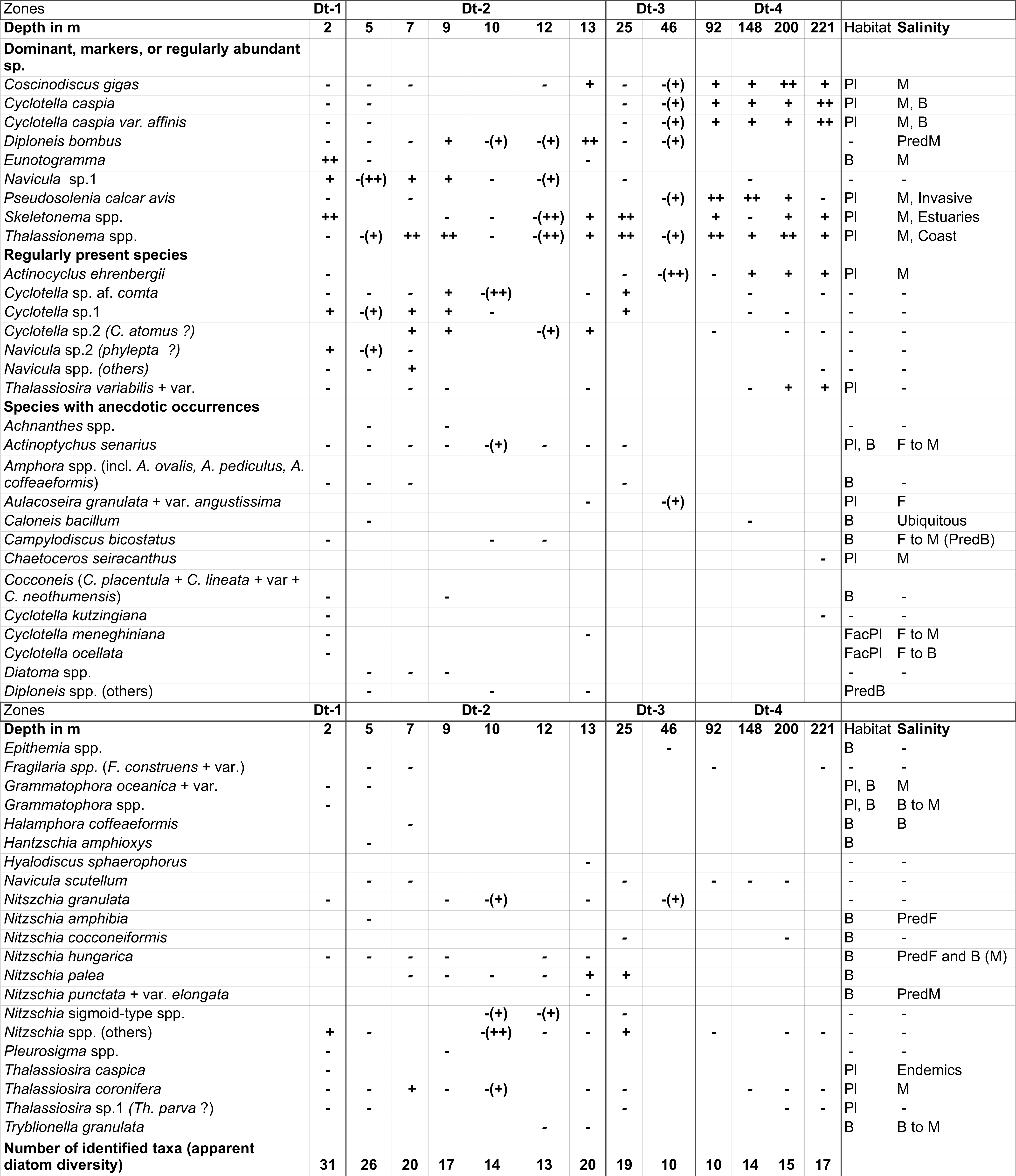
42The ¹⁴C/¹²C and ¹³C/¹²C ratios were measured by accelerator mass spectrometry (AMS) at the ¹⁴CHRONO Centre, Queen’s University Belfast. The sample ¹⁴C/¹²C ratio was background corrected and normalised to the HOXII standard (SRM 4990C; National Institute of Standards and Technology). The radiocarbon age and one standard deviation were calculated using the Libby half-life of 5568 years following the methods of Stuiver & Polach (1977). F¹⁴C is calculated according to Reimer et al. (2004). The radiocarbon ages and F¹⁴C were corrected for isotope fractionation using the AMS measured δ¹³C, which accounts for both natural and machine fractionation. Post-bomb reservoir offsets, sometimes called reservoir ages, are calculated using the F¹⁴C of the sample and that of the reservoir where the carbon is obtained (Keaveney & Reimer, 2012; Soulet et al., 2016), in this case the atmosphere from the year the samples were collected. Reservoir offsets (R) were calculated relative to the atmosphere (in 2012) using the following equation:

43-8033*ln(F¹⁴C_sample/ F¹⁴C_atm)

44where F¹⁴C_atm ± F¹⁴C_sigma = 1.04036 ± 0.0020 (Levin et al., 2013).

45The uncertainty in the reservoir offset (σR) was calculated from the uncertainties in the radiocarbon age of the sample (σ_sample) and the atmosphere (σ_atm) combined in quadrature using the following equation:

46σR = √ (σ_sample² + σ_atm²) where

47σ_atm = -8033*ln [(F¹⁴C_atm) + (F¹⁴C_sigma)] +[8033*ln (F¹⁴C_atm)]

3.11. δ¹³C_carbonate and δ¹⁸O_carbonate

48The stable isotope composition of carbonate shells varies with specific environmental conditions such as water temperature, freshwater supply and productivity (e.g. Wefer & Berger, 1991; Weinelt et al., 2001). Three different taxonomic groups have been selected for stable isotope measurements: ostracods, benthic foraminifers and bivalve remains. For the isotopic study of ostracods and benthic foraminifers, different species were grouped together since no single species occurred throughout all samples in sufficient numbers. For bivalve remains, a distinction at species level was not possible due to strong fragmentation.

49At the Leibniz Institute, mollusc shell material was ground with an agate mortar. Approximately ten ostracod valves as well as foraminiferal tests were picked per sample and ~100–400 µg of each sample material were put into a clean 10 ml exetainer vial. After sealing the exetainer vial with a septum cap (caps and septa for LABCO exetainer 438b), the remaining air was removed by flushing the vial with He (4.6) for 6 minutes at a flow of 100 ml per minute. After flushing, ~30 µl of anhydrous phosphoric acid was injected through the septum into the sealed exetainer using a disposable syringe. After ~1.5 h of reaction time, the sample was ready for isotope measurement.

50The oxygen and carbon isotopic composition of the CO₂ in the headspace was measured using a Thermo Finnigan GASBENCH II coupled online with a Thermo Finnigan Delta V isotope ratio mass spectrometer. Reference gas was pure CO₂ (4.5) from a cylinder calibrated against the Vienna PeeDee Belemnite (VPDB) standard by using IAEA reference materials (NBS 18, NBS 19). Isotope values are shown in the conventional delta-notation (δ¹⁸O) in per mil (‰) versus VPDB. Reproducibility of replicate measurements of lab standards (limestone) is generally better than 0.10‰ (one standard deviation) (Gilg et al., 2003).

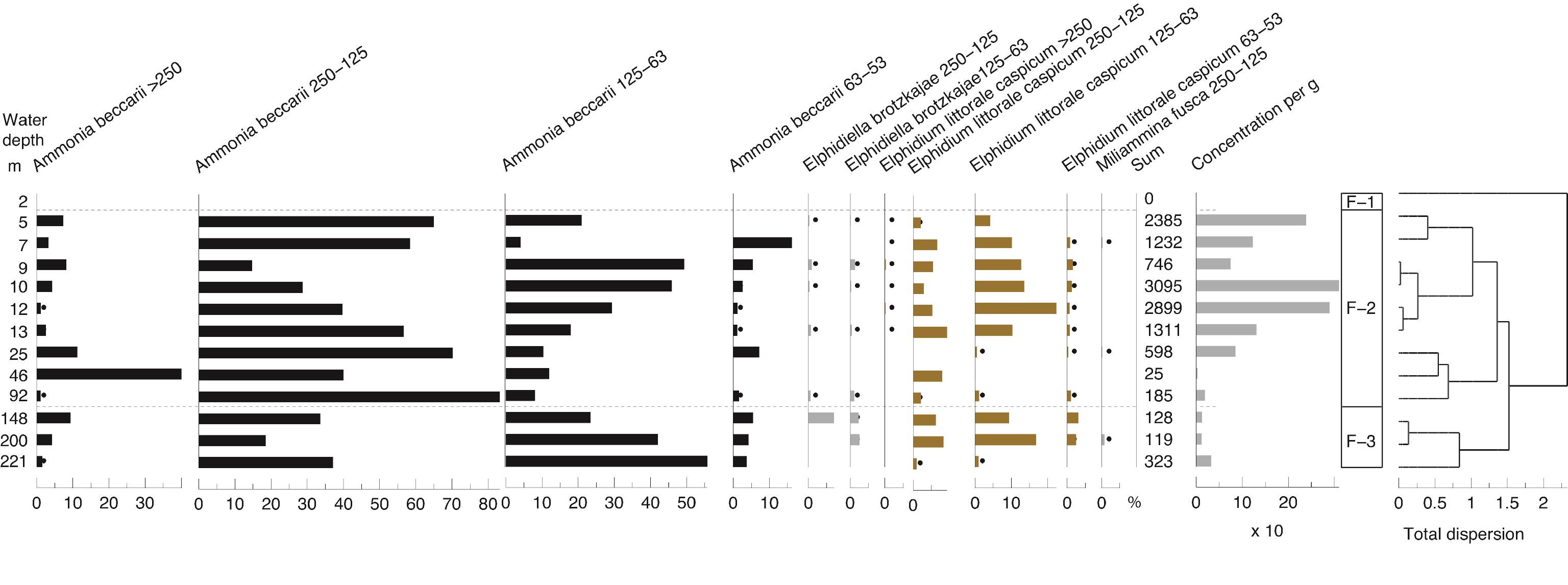
4. Results

4.1. Oceanographic data

51Water depths remain shallow over a long distance (>~30 km) in the eastern part of the study area and consequently the sampling stations are far apart. It is not until ~46 m water depth that a significant depth change occurs with the shelf break. Then the westernmost and last four stations are on a steep slope and closer together with the last station being at 221 m, therefore not reaching the abyss (Fig. 1C).

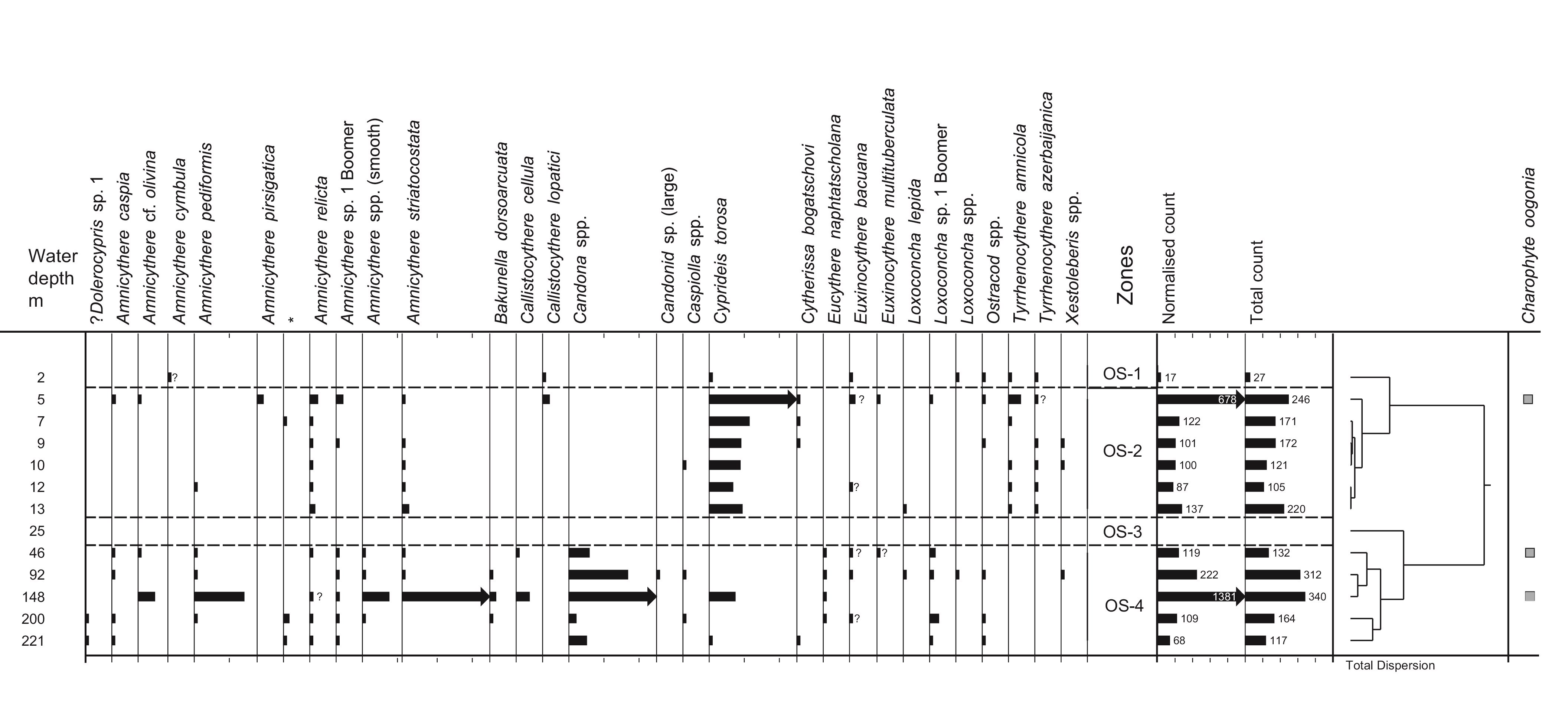
52The surface water temperature increases westward from 6.5 to 11.5 °C and is the most variable parameter measured along this transect (Fig. 2B). Temperature in the water column is uniform in the shallow waters of transect A. However, at the deeper stations, the bottom temperature ranges between 6 and 11 °C with the highest temperatures at ~46 m. In the water column, a weak thermocline occurs at 80–160 m. An anomaly in the water structure is visible at station 5 (10 m water depth). From remote sensing, winter surface temperature varied between 11 °C near the coast and 15 °C offshore (Table SI 3). In addition, summer surface temperature estimates were obtained too: 31 °C near the coast and 28 °C offshore that correspond well to the fact that the SE corner of the Caspian Sea is usually the warmest of the whole water body (Table SI 3).

53Figure 2. Oceanographic data for the two parts of the transect: A and B in February 2014. 2A: Vertical distribution of Chl-a. Data are plotted against station numbers and distance between stations (Table SI 1). See Table SI 2 for units of the parameters measured. Analyses: S. Sanjani. 2B: Vertical distribution of Temperature, Salinity, Sigma-T (see Fig. 2A). 2C: Vertical distribution of pH, DO2 and Turbidity (see Fig. 2A).

54Other parameters are fairly constant: the surface and bottom salinities hardly change and remain around 11.9 psu, except in the two shallowest sites (stations 1 and 2) where they rise to 12.8 psu (Fig. 2B). Density values at the surface layer decrease from δt = 9.55 in the eastern part, in front of the Gorgan bay inlet, to δt = 8.62 in the western part of the surveyed area (Fig. 2B). At the westernmost deepest station (station 8), density goes up from δt = 8.62 at the surface to δt = 12.25 at the bottom. The pH values are between 8.5 near the coast and 7.9 at 200 m depth with a drop between 80 and 90 m (Fig. 2C). The dissolved oxygen content (DO₂) also varies little, i.e. between 10.8 ppm at the surface and 6.3 ppm at depths with a steep gradient between 80 and 100 m (Fig. 2C). Turbidity is generally low between 1 and 6 Formazin Turbidity Units (FTU; Fig. 2C), and it decreases from east to west. At the bottom of the shallowest site (station 1; 2 m depth) in front of the Gorgan River, the turbidity rises to a maximum of 16 FTU. Chl-a values are low between 0.2 and 1.5 µg/L, with higher values in station 11 (maximal depth of profile 92 m) at 17 m water depth (Fig. 2A). The Chl-a value decreases to 0.15 µg/L at the depths of 15 to 100 m and then constantly remains at 0.1 µg/L for the depths >100 m. The remotely sensed Chl-a values show a downtrend from the shallow near-shore waters to the deeper off-shore areas (Table SI 3).

4.2. Sedimentology

55The sediment at most stations is silty with 5–15% clay with a maximum of 20% at 12 m (zone S-3) (Fig. 3). Only samples at 5 and 7 m contain significant amounts of sand, i.e. 14 and 44% respectively (zone S-2). Organic content is 5–10% and increases slightly with depth. Carbonate content varies from 8 to 23%. WC increases with depth and seems to run parallel to the amount of organic matter; but it seems to be inversely related to the amount of sand. In general, the overall curve of the MS values clearly shows the highest values in samples at 7 and 9 m water (zone S-2).

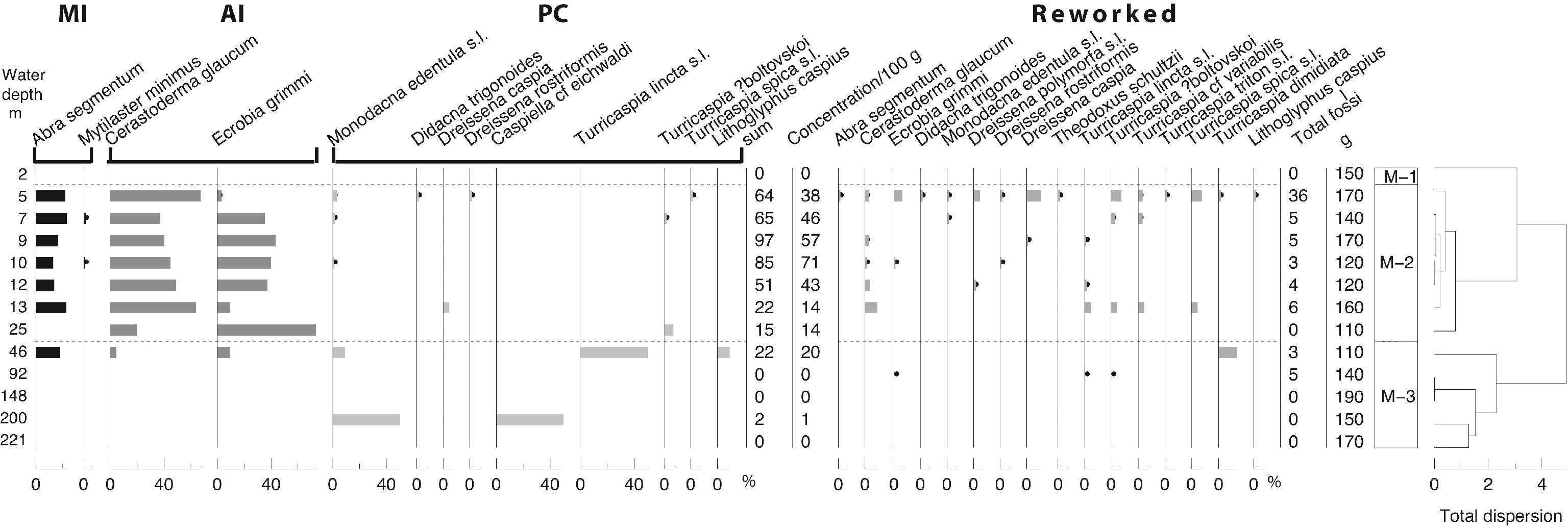
56Samples tested at 12 and 148 m both contain a significant quantity of tephra (Fig. SI 2). Shards at 148 m are mainly colourless and chunky to plate-like in form, but light brown and fluted shards are also present. Shards in the 12 m sample are also predominantly colourless, but are slightly more vesicular. A high proportion of shards in both samples show signs of abraded edges (e.g. Fig. SI 2: no 7, 14) and in some instances, pitted surfaces are evident.

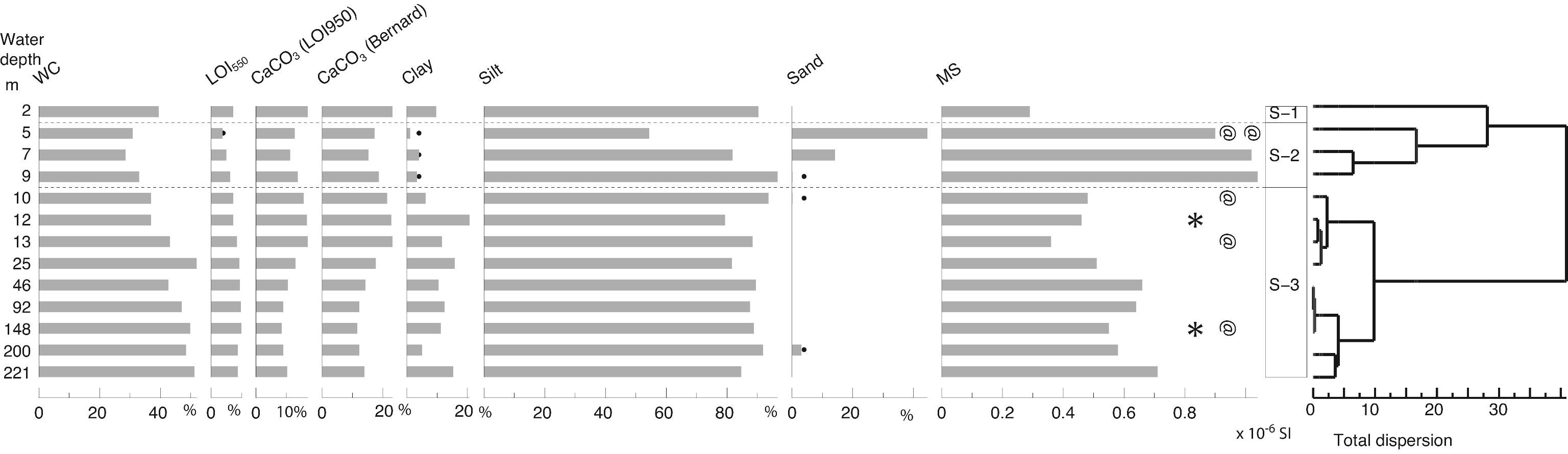
57Figure 3. Sedimentology. WC: water content, LOI: Loss-on-Ignition, MS: magnetic susceptibility. Analyses: P. Habibi, F. Chalié and S. Haghani. Black dots for low values. * for the location of the two tephra samples and @ for the 14C samples.

4.3. Palynology: pollen, NPPs and dinocysts

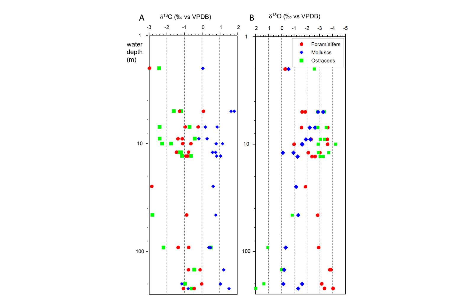
58Zonation of the pollen, spore and non-pollen palynomorphs (NPP) has been performed separately from zonation of the dinocysts. The two zonation schemes show significant differences; because the pollen zonation represents changes on land and the dinocyst zonation reflects changes at the water surface (Fig. 4).

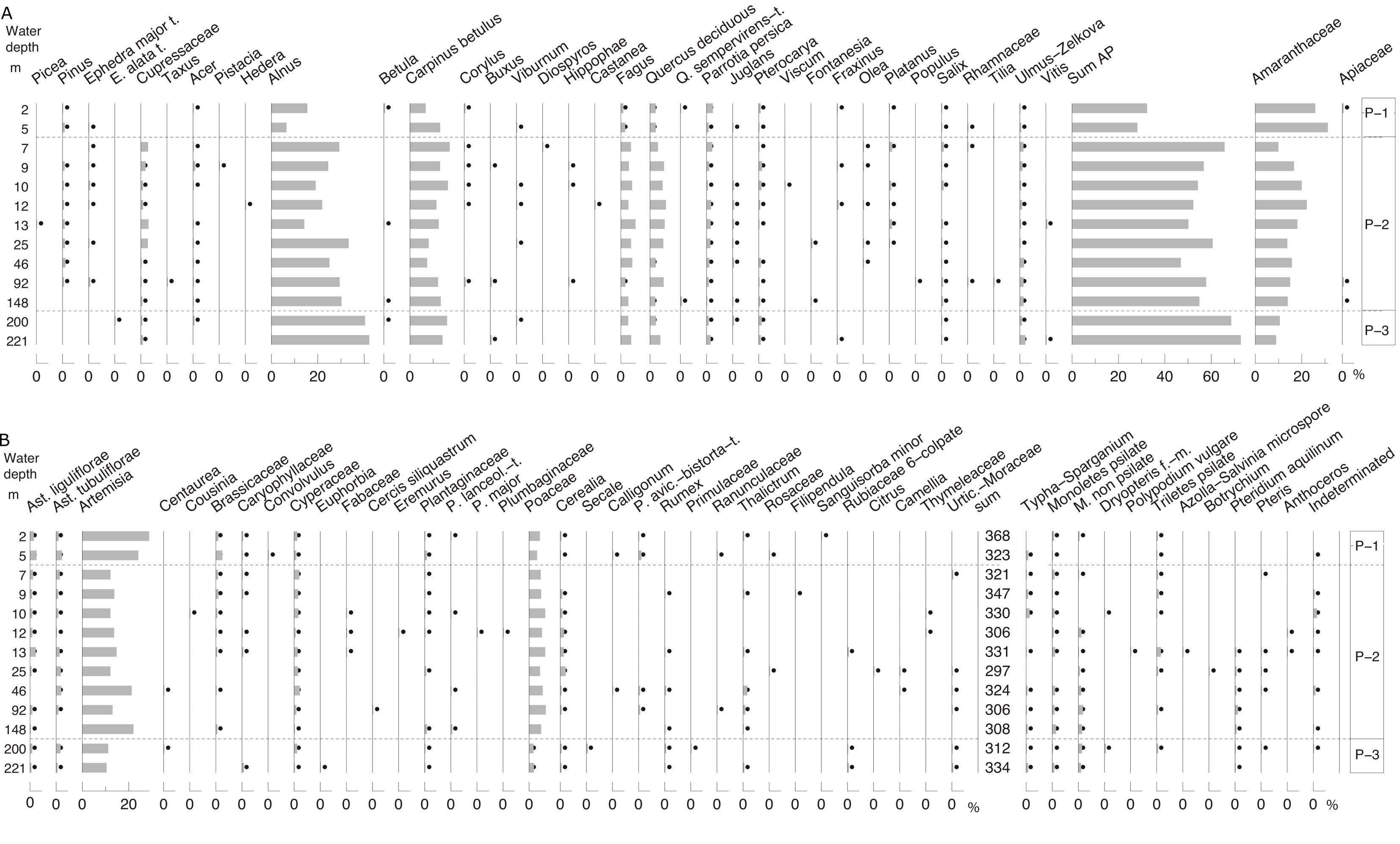
59Figure 4. Palynology (%). Black dots for values <0.5%. Stars in X axis when absolute abundance in number of specimens per g of wet sediment. Analyses: S.A.G. Leroy. 4A, 4B and 4C: pollen and NPPs, 4D: dinocysts and foraminifer linings.

60The samples are moderately rich in pollen and spores, with absolute abundances between 4800 (7 m) and 17,600 (46 m) palynomorphs per ml of wet sediment. The palynomorphs are well preserved with few, but continuously present, reworked ones displaying a small maximum (7%) at 200 m.

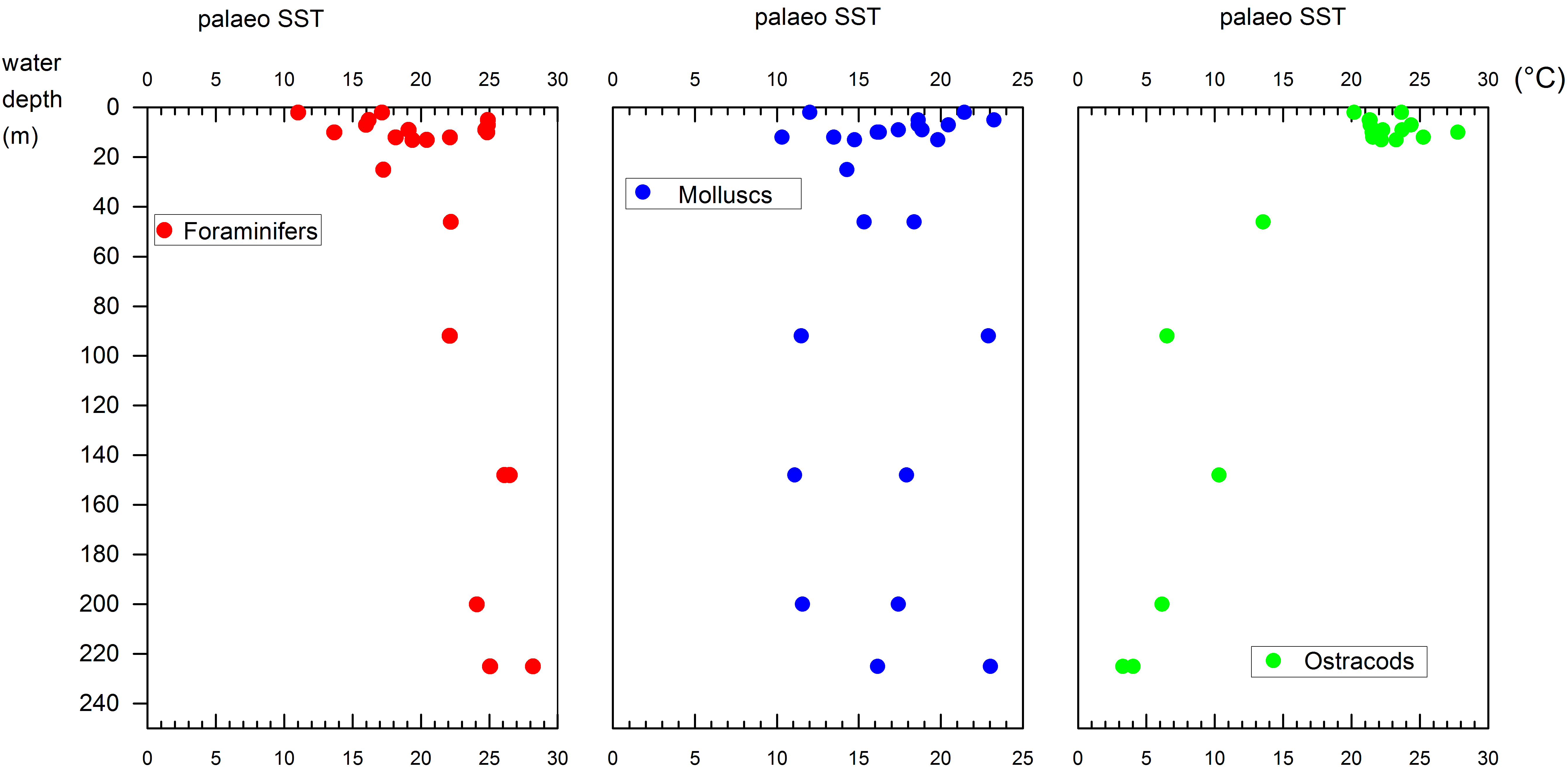
61Zone P-1 (2 to 5 m): Alnus dominates (7 to 15%) the arboreal pollen (AP). Other AP components are Carpinus betulus, Fagus, Quercus, Parrotia persica (Fig. SI 3: 1-2), Juglans, Pterocarya (Fig. SI 3: 3) and Ulmus-Zelkova (Fig. SI 3: 4-5). The Amaranthaceae and Artemisia percentages are maximal, respectively >25% and >24%. Highest values of Botryococcus are at 2 m. Fungal spore percentages are very high at 5 m and low at 2 m. Glomus peaks at 5 m.

62Zone P-2 (7 to 148 m): Alnus percentages almost double that seen in zone 1. The most significant change in the non-arboreal pollen (NAP) is the decrease of Amaranthaceae and Artemisia. Fungal spores are abundant.

63Zone P-3 (200 to 221 m): Alnus present the highest percentages of the transect (40%). AP percentages are maximal (70%), synchronous to an increase in a wide range of arboreal taxa belonging to the Hyrcanian forest flora. NAP values are at their lowest and consist of Amaranthaceae, Artemisia and Poaceae. At 221 m, a slight increase of Anabaena (Fig. SI 4: 1-2), Pterosperma and incertae sedis 5b (Fig. SI 4: 3-5) is noted. These taxa are typical of the Caspian Sea offshore (Leroy et al., 2007, 2013c, 2014). Fungal spores are abundant.

64All samples are rich in dinocysts with absolute abundances varying between 1800 (station 2, 5 m) and 8800 (station 7, 13 m) cysts per ml of wet sediment. The absolute abundance of the foraminiferal linings (Fig. SI 3: 11) varies from 0 to 6400 specimens per ml.

65Zone Dc-1 (2 m): Lingulodinium machaerophorum (Fig. SI 4: 9-13) and Impagidinium caspienense (Fig. SI 4: 6-8) are dominant with respectively 56 and 38%. Pentapharsodinium dalei reaches maximal values of 2%.

66Zone Dc-2 (5 to 25 m): L. machaerophorum is largely dominant with percentages above 65%. I. caspienense is around 17%. Some occurrences of Caspidinium rugosum, C. rugosum rugosum and Spiniferites cruciformis are observed. Foraminiferal linings are abundant in the shallow stations and steadily decrease with depth.

67Zone Dc-3 (46 to 221 m): I. caspienense dominates with values often >50%. L. machaerophorum percentages (both form B and form s.s.) drop significantly to around 30%. Brigantedinium is continuously present with its highest values at the deepest station. Spiniferites belerius and P. dalei cysts are frequent. Foraminiferal linings have are rare.

68The P/D ratio should in theory decrease with the increasing distance to the coast, but this is not the case. Perhaps because the depth transect does not divert much away from the coast.

4.4. Diatoms

69Table 1 provides a list of the diatom species encountered with their semi-quantitative estimated abundance and ecological preferences. Figure SI 5 depicts the most abundant and/or characteristic diatom marker species. Diatoms are sparse; but valve preservation is quite good (Table 1). Deterioration is mainly due to of the breakage of the frustules of larger cells (e.g. Coscinodiscus spp. and Actinocyclus spp.), and consists of valves breakage. Exceptionally, samples at 13 and 221 m yielded valves with some largely dissolved features. Except for a few valves in these two samples, the shape of most of the valves is sufficient for identification.

70Table 1. List of diatom species and their semi-quantitative occurrence: -: rare ; +: present ; ++: relatively abundant (even for poor samples); -(++): rare in the sample, but dominant within the assemblage; Pred = Predominantly.

71For species habitat: Pl = Planktonic; B = Benthic; FacPl = Facultative Planktonic; For salinity preferences: F = Freshwater; B = Brackish; M = Marine. Analyses: F. Chalié.

72Of the dominant diatoms, most of the planktonic species are mainly found in the deeper locations, while the benthic species are represented in greater abundance in the areas close to the coast, i.e. in shallower waters. This is also observed for less well represented species (e.g. Nitzschia spp., Actinocyclus spp.), despite some exceptions (e.g. Thalassionema spp.).

73The number of identified taxa in each sample provides an approximate measure of diversity, since some taxa refer to a group of several species found with low percentages or which are identifiable to the genus level only (e.g. Amphora spp.). This apparent diversity is consistently high at sites near the coast (zones Dt-1 and 2, depth <12 m), decreasing only slightly with increasing depth. Apparent diversity slightly increases again at 13 and 25 m, then reaches its lowest values at 46 and 92 m, and tends to increase towards deeper (offshore) sites. Thalassionema spp. and Thalassiosira spp. are found all along the transect.

74The transect can be divided into four distinct diatom zones:

75- Zone Dt-1 (2 m) is characterized the highest apparent diversity of the transect and by an assemblage of Eunotogramma spp., which are seen only sporadically at deeper sites.

76- Zone Dt-2 (5-13 m): Assemblages in this zone typically contain Cyclotella spp., excluding C. caspia, Actinoptychus senarius, Navicula spp. and Nitzschia spp.). P. calcar avis is almost absent. Skeletonema spp. and Diploneis bombus are also present, mainly in the deeper part of the zone.

77- A major change in the composition of the assemblages is observed between 25 and 46 m (zone Dt-3). Actinoptychus senarius, found between 2 and 25 m, disappears; while Actinocyclus ehrenbergii appears at 25 m and is present in deeper samples. The sample from 25 m contains a mixed assemblage, resembling samples from both the shallower and the deeper parts of the transect. This results in an intermediate assemblage, containing both species mainly found at sites with lower water depth (e.g. A. senarius, C. sp. af. comta) and species predominantly occurring in deeper sites (e.g. A. ehrenbergii, C. caspia and P. calcar avis). The sample at 46 m contains diatoms species of large size (A. ehrenbegii, C. gigas, D. bombus), but with very low abundance.

78- Zone Dt-4 (46 to 221 m) is characterised by more typically brackish to marine species (e.g. A. ehrenbergii, P. calcar avis and C. gigas). This deeper part of the transect is also marked by the disappearance of A. senarius, and from 92 m, of D. bombus, both speciesconsistently present at shallower sites. An abundance of the invasive species P. calcar avis (Karpevitch, 1975 in Karpinsky, 2010) also characterizes this zone, with a maximum representation recorded at 92 and 148 m.

4.5. Foraminifers

79Four benthic species were identified: Ammonia beccarii, Elphidium littorale caspicum, Elphidiella brotzkajae and Miliammina fusca. Of these four, E. littorale caspicum and E. brotzkajae are endemic species. Foraminifers are absent in the shallowest sample (2 m) (Fig. 5); but are abundant from 5 to 25 m, becoming rare at greater depths.

80Figure 5. Foraminiferal tests (%) with sizes in µm. Black dots for values <0.5%. Analyses: P. Habibi.

81Three zones mostly mainly characterised by a change in the size of A. beccarii have been established. In zone F-1 (down to 13 m), small A. beccarii and small E. littorale caspicum are observed. In zone F-2 (25 to 92 m), the size of these main foraminifers slightly increases. Zone F-3 (92 to 221 m) contains the same two dominant species; but with, in addition, a significant number of E. brotzkajae.

4.6. Ostracods and charophytes

82All samples, except one from 25 m that was barren, yielded ostracods and had total abundances ranging between 17 (station 1, 2 m) and 1381 (station 10, 148 m) specimens per 100 g of wet sediment (Fig. 6). Reworked specimens were generally rare, but most common at 2 m (not shown on figure). Broken fragments were common in most samples but whether this damage was due to recent sediment transport or to subsequent sample preparation is not known. Figures SI 6A and SI 6B depict the key species recovered.

83Figure 6. Distribution of ostracods and charophytes without reworked specimens. Individual ostracod species abundance (scale tick = 100 specimens) and counts shown normalised for 100 g of wet sediment and total counts; valves = black, carapaces = grey; cut off for species = 250; cut off for normalised and total counts = 500. Charophytes shown if present (grey squares). Analyses: J. Athersuch.

84Ostracods have a clear depth distribution along this transect with four distinct assemblage zones being recognised. Zone O-1 (2 m) is characterised by the least abundant and diverse ostracod fauna of all the samples and includes rare occurrences of Callistocythere lopatici, Amnicythere ?cymbula and small forms of Tyrrhenocythere spp.

85Zone O-2 (5 – 13 m) is dominated by Cyprideis torosa. Juvenile specimens are without exception clearly noded (2-3 nodes) whereas in adults, nodes are either absent or poorly developed. The peak occurrence of this species is at 5 m, below which abundance generally declines with increasing depth to 13 m. This species is virtually absent in samples from greater depths with the exception of 148 m (discussed below). Other species also occur, but are far less abundant. These include Callistocythere lopatici, Tyrrhenocythere amnicola, T. azerbaijanica, Amnicythere striatocostata and Euxinocythere relicta. At 5 m additionally a number of rare species are present, mainly Callistocythere spp.and Amnicythere spp.

86The sample from 25 m (zone O-3) lacks ostracods. The assemblages of zone O-4 (46 to 221 m) are dominated by Candona spp. Other, very much rarer, species in this zone include Bakunella dorsoarcuata, Eucythere naphtatscholana, Callistocythere cellula and a number of Amnicythere spp., typically including A. caspia and A. pediformis. The sample at 148 m is exceptional in that in addition to Candona spp., it yielded common specimens of C. torosa and the most abundant occurrences of several other species (e.g. A. striatocostata, A. pediformis, A. cf olivina). Charophyte oogonia occurred very rarely at several locations between 5 and 200 m.

4.7. Molluscs

87No molluscs were noted in the sample at 2 m (zone M-1; Fig. 7). In zone M-2 (5 and 25 m; Fig. 7 and Fig. SI 7), samples contain abundant molluscs and are dominated by Cerastoderma glaucum, Ecrobia grimmi and Abra segmentum. Endemic Caspian species are very rare. The absolute abundance of fresh shells is high to very high from 5 to 12 m. In zone M-3, the sample from 46 m has low numbers of shells but the fauna is dominated by relatively well-preserved endemic (Pontocaspian or PC) gastropods (especially Turricaspia lincta s.l.). Molluscs are almost lacking from 92 m downwards.

88Figure 7. Molluscs (%). Left: in-situ specimen, right reworked specimen. Analyses: F. Wesselingh. Molluscs from the Gorgan transect. S.l. denotes sensu lato (in the broad sense). MI is modern (20th century) invasive species, AI is ancient (Early Holocene) invasive species, PC is Pontocasian species.

89Ancient invasive species (AI) dominate the entire fauna followed by modern invasives (MI). Fresh shells of endemic species are rare and lacking in most samples. Endemics are relatively abundant at only 46 m. The numbers of reworked specimens are generally low (0–14%) with the exception of the sample from 5 m (56% fossil material with extensive signs of abrasion) and the sample from 13 m (27%).

4.8. Stable carbon and oxygen isotopes of carbonates

90The distribution of carbon and oxygen isotopes versus water depth in foraminifers, ostracods and mollusc shells is displayed in Figure 8. For the carbon isotopic composition (Fig. 8A), no trend is observed with respect to water depth in foraminifers, ostracods or molluscs. However, a general offset in δ¹³C of ~1‰ is detected between the taxonomical groups. Molluscs show the highest δ¹³C around 0.8 (± 0.87) ‰, foraminifers are intermediate around -0.99 (± 0.76) ‰, whereas ostracods show the lowest δ¹³C around -1.37 (± 0.89) ‰ (Fig. 8A).

91Figure 8. 8A: Carbon isotopes of carbonates. 8B: Oxygen isotopes of carbonates. The depth axis is in log scale. Analyses: U. Struck.

92In the case of oxygen isotopes, the three taxonomical groups show various behaviours with increasing water depth (Fig. 8B). Ostracods in shallow water samples show low δ¹⁸O around -2.10 (± 1.86) ‰. Values increase progressively below 10 m water depth to 2‰ at 221 m. Foraminifers show the opposite trend starting with high δ¹⁸O around -0.37 ‰ in shallow waters while decreasing to low values down to -4.03‰ in samples from the greatest water depths (Fig. 8B). Molluscs show a variable distribution of δ¹⁸O at intermediate values -1.67 (± -0.96) ‰ (Fig. 8B).

93A reconstruction of the ambient water temperatures with an oxygen isotope based palaeo-temperature equation (Epstein et al., 1953) has been applied on the isotopic results on hand by using existing δ¹⁸O data from the Caspian Sea water bodies (Froehlich et al., 1999) and the δ¹⁸O data from the calcareous taxonomic groups (Fig. 9). Typical water temperatures in the Caspian Sea show strong vertical differences. The upper 30 to 50 m of the water column show temperatures with strong seasonal fluctuation around 20 to 25 °C (Froehlich et al., 1999). Below 50 m the waters show very small temperature variations around 5 to 6 °C. This pattern is best reflected in the reconstructed temperatures from the benthic ostracods whereas molluscs and foraminifers show no such clear depth-related pattern (Fig. 9).

94Figure 9. Reconstructed modern Caspian Sea water temperatures (reconstructed-SST) versus water depth based on the δ18O composition of biota groups and the ambient δ18O composition in the surrounding water (Froehlich et al., 1999). The resulting depth distribution of reconstructed SSTs reflects the actual water temperatures best when related to ostracod-derived SSTs.

4.9. Radiocarbon dating

95The dates on the shells of the mollusc Cerastoderma glaucum from 5, 10 and 13 m gave post-modern ages and F¹⁴C values higher than the current atmospheric value which results in theoretically impossible negative reservoir offsets (Table 2). Therefore no reservoir offsets are given for these samples. The ostracod sample at 148 m was small (0.2 mg carbon), and may derive from transported material (further discussed below) so is not considered reliable. The reservoir age (R) for the ostracod sample at 5 m was calculated relative to the atmosphere (in 2012) as 747 ± 29 yr.

96Table 2. Results of the 14C measurements including the laboratory number, sample identification, species, depth, radiocarbon age, error, F14C, and one standard deviation in F14C. Analyses: P. Reimer. * calibrated with CALIBomb (Reimer & Reimer, 2018) using the IntCal13 calibration dataset (Reimer et al., 2013) and for >modern samples the Northern Hemisphere calibration dataset extension (Levin & Kromer, 2004; Levin et al., 2013) with 1 year smoothing.

5. Interpretation

5.1. Oceanography

97The highest salinities in the shallowest sites are most likely due to very high evaporation over the very warm water that is adjacent to a semi-desert. Station 1 (2 m) is influenced by varying combination of the outflow of the perennial Gorgan River, which is especially small in February (low salinity component), and by the outlet of the shallow Gorgan Bay (high salinity component of 13.1 to 14.3 psu in April 2011; Habibi, 2013). The most significant characteristics in this station, particularly at the base of the profile, are the high turbidity with cold and saline waters.

98For explaining the anomaly at station 5, the eastern dense and saline water of the south basin, which has a low temperature, had probably sunk. When it came in contact with a deep and denser water at station 5, the first one overlaid the second (Fig. 2B). The bathymetry with a small shelf would have facilitated this flotation, as well as the northerly winds.

99Regarding Chl-a levels,in general it is known from Nezlin (2005) that the Chl-a levels should be higher in summer than in winter; but our limited data suggest otherwise (Table SI 3).Moreover the values of the shallow point at station 1 (2 m) may be overestimated due to errors resulting from the effects of reflectance of adjacent land areas (Table SI 3).

5.2. Sedimentology

100The silty sediment at the shallowest site (2 m) is influenced by the discharge of the Gorgan River (Lahijani et al., 2008) and by the outlet of Gorgan Bay. Further away from the river mouth (5–7 m), bottom sediments are resuspended in the wave-breaking zone, winnowing of the finer grains that are relocated outside the zone. This creates a narrow sand strip between muddy sediments along the south-east coast. The estimated fair-weather wave-breaking depth of 3.8 m explains why at a depth around 5–7 m, more sand is found (Figs 3 and 9). The shallow waters and the coarser grain size indicate that the current shore face facies extends down to 7 m, perhaps 10 m maximum. The above situation corresponds to the contemporary water level. This sand body must have moved shorewards when the water level was slightly higher in 1995 and receded when the water level was significantly lower in 1977.

101The sediment composition (based on LOI) is fairly similar (containing about 20% of carbonates) to four short cores taken offshore in the southern basin of the Caspian Sea: CS10 offshore Babolsar, US01 offshore Turkmenistan, CS03 offshore Anzali and US02 in the centre of the basin (Leroy et al., 2013b). The main differences are that the Gorgan transect is richer in organic matter and poorer in clay.

102A comparison of the sediment to that along three shallow transects between on each side of Babolsar (Sadough et al., 2013; Ghane et al., 2014) indicates that the grain size is fine sand in the shallower depths, becoming finer at 15 and 20 m. Larger grain sizes were found here in front of rivers. LOI₅₅₀ is between 1 and 12% and CaCO₃ between 1 and 6.6%.

103The varied morphology and colour of many of the tephra shards suggests that they are predominantly reworked. Given the proximity of the Caspian Sea to many active volcanoes in the Alborz (Damavand) (Davidson et al., 2004) and Caucasus (Ararat) (Karakhanian et al., 2003), and systems known to have been active in the last millennia (Mt Elbrus and Kazbek volcanoes in the Great Caucasus, Global Volcanism Programme, 2013), as well as the eastern Mediterranean, tephra in the Caspian Sea sediments is potentially derived from a large area. Without geochemical analyses of the tephra, its precise source cannot be determined. Its presence nevertheless shows that the sampling site is within the catchment of one or more volcanic systems, and that therefore potential to apply tephrochronology in this area exists. Primary airfall deposits in a sedimentary sequence can be distinguished from background detrital material using absolute abundances, morphology and geochemical analyses of shards (Gatti et al., 2013).

104The south-east corner of the CS has unique characteristics; it is a transition zone from arid to humid subtropical climate, from wave- to river-dominated coast, from carbonate to siliciclastic sediments, from deep gently-sloping to steep-sloping shelf and an area with two sets of approaching coastal and offshore currents in the nearshore and deeper parts respectively. The signature of the above mentioned factors are reflected in the water column properties, bottom sediments and organisms. Water with high turbidity induced by the Gorgan River and coastal currents expand in the wide shallow coastal area. They are the main source of muddy sediments in the coastal zone. Breaking of the incoming waves first happens at a depth of around 4 m, flushing out fine detritics and resulting in a belt of sands. Transported sediments from fluvial systems and coastal currents are rich in carbonate. Moreover shallow waters in an arid climate are favourable for carbonate precipitation, from both biogenic and chemical sources. They also cause low MS value in the sediments by dilution.

5.3. Palynology: pollen, NPPs and dinocysts

105The pollen assemblages are directly influenced by the vegetation in the coastal plain as well as on the northern slopes of the Alborz Mountains. In particular the influence from the dry eastern part with desertic, semi-desertic and steppic conditions is demonstrated in zone P-1. In this zone, a minor influence from the Gorgan River can be seen in the presence of Botryococcus (indicating eutrophication) and the abundance of fungal spores. In zones P-2 and 3, the regular increase in arboreal elements reflects the westwards distribution of the Hyrcanian forest and the westward increase in precipitation.

106Regarding the dinocyst data, samples shallower than 25 m (zone Dc-2) are dominated by L. machaerophorum and the deeper ones (zone Dc-3) by I. caspienense, with the exception of one sample at 148 m. This clear change indicates that the shift is mainly related to distance to the coast. The Gorgan assemblages of zone Dc-2 resemble the high salinity surface samples from the Caspian Sea and surrounding areas, as well as three more coastal cores out of the four short cores published (Fig. 1B; Leroy et al., 2013b). Zone Dc-3 with lower L. machaerophorum values resembles the assemblages of the last 3000 years of the sequence TM, which was taken in a coastal lagoon north of Gorgan (Fig. 1B), from which it was suggested that temperature was the leading driver of the development of L. machaerophorum (Leroy et al., 2013b).

107Pyxidinopsis psilata, a taxon frequent in low salinity assemblages of the Late Pleistocene and Early Holocene in the Caspian Sea, is absent (Leroy et al., 2007, 2013c, 2014); Spiniferites cruciformis, another taxon of low salinity, has rare occurrences between 9 and 46 m. The deepest station is characterised by Anabaena, Pterosperma and incertae sedis 5b, taxa that are also abundant in the long cores GS05 and GS18 and the short cores CP14, CP18 and CP21 of the deep basins (Leroy et al., 2007, 2013c, 2014) indicating that these taxa are good indicators of offshore waters. Finally the sample at 5 m, which is very sandy, also contains the lowest abundances of dinocysts and the highest abundances of foraminiferal test linings. As expected it is one of the samples with high absolute abundances of foraminiferal tests too.

108The unexpectedly high values of the P/D ratio in zone Dc-3, when it should be at its lowest, are partly due to the increasing density of the vegetation cover westwards, as well as the increasing occurrence of Alnus swamps along the coast westwards (Leroy et al., 2013a). Removal of Alnus pollen, an over-represented tree, from the ratio calculation did not, however, reverse this trend.

5.4. Diatoms

109Four distinct assemblages were identified along the depth profile (Table 1) with the main change occurring between 25 and 46 m.

110Apparent diversity seems to be an indicator of proximity to the shoreline, which in this case is directly related to water depth. Diversity of the habitats and the variety of ecological niches are certainly greater at the shallow sites. As expected, benthic species are rather more abundant in the shallower sites, and their abundance decreases offshore, especially from 25 m.

111Invasive species are more abundant, at times even dominant, in some of the offshores sites. In shallower sites (i.e. near the shore), in contrast, they appear to be less abundant, or even absent. Ecological diversity, as mentioned above, and species competition could account for this differential dominance in P. calcar avis, along the transect.

112One of the main limitations of diatom data used to reconstruct water salinity in the Caspian Sea is that most species behave as euryhaline species. Some marine species have developed to tolerate the freshwaters of the Northern Caspian basin, and most of them are adapted to the current range of salinity (Proshkina-Lavrenko & Makarova, 1968; Genkal, 1992), much better than in the sea (Karayeva & Makarova, 1973). In our samples, salinity cannot be considered a controlling factor in diatom distribution, since it is almost constant. The ecological preferences of diatoms are rarely well understood for parameters other than salinity. However, one may speculate that the eurytopicity of diatom species shown for salinity could extend to other environmental variables. This is a common consequence of the Caspian history and gradual variations of some parameters along the Caspian sub-basins. This suspected adaptation makes the interpretation of the diatom distribution fuzzy in terms of environmental gradients.

5.5. Foraminifers

113Fine sediments and their organic matter content on the bottom are the main influencing factors for benthic foraminifers (Hermelin & Shimmield, 1990). Many foraminifers have various microhabitats in the upper layer of sediment, moving vertically for nutrients (Linke & Lutze, 1993). The distribution of foraminifers could reflect productivity in water and exchange between water masses. In the Caspian Sea, the limit for benthic foraminifer occurrence is no more than 50 to 70 m. This fits well with our observations that show a clear drop in absolute abundances of carbonate tests and organic test linings between 25 and 46 m. In this study, the low numbers of foraminifers in samples deeper than 50 m is clearly due to reworking.

114The same four species occur recorded in this study plus Cornuspira spp. Occurred in a shallow Usnel box core US01 (13 m water depth) (Leroy et al., 2013b). The same absolute abundances occur in this core and in the samples from 10–12 m in the transect, i.e. 300 tests per g.

115In a springtime study of six offshore transects west and east of Babolsar to a maximal depth of 20 m, an Ammotium species was also found but Elphidiella was not recorded (Sadough et al., 2013; Ghane et al., 2014). In that study, the absolute abundance of benthic foraminifers was found to increase with decreasing grain sizes. In the Gorgan Bay for comparison, in addition to the four identified species by the current study, Habibi et al. (2013) also reported two more species: Cornuspira spp. and Discorbis aguajoi. This was in core PH01 from middle of the bay in a water depth of 3.8 m. The abundance of those euryhaline foraminifers in the Gorgan Bay could be related to the frequent salinity changes, the great availability of nutrients, as well as the numerous water-level fluctuations affecting the size of the bay.

5.6. Ostracods and charophytes

116On the basis of Gofman’s work, Yassini (1986) was able to distinguish seven ostracod assemblages all of which appear to have been strongly depth-related. These assemblages grouped into nearshore and offshore environments with a boundary at about 100 m that can be approximately equated to the boundary between zones O-2 and O-3 (Fig. 6) described herein. However, depth may not be the primary control as, not surprisingly, there is much evidence in Gofman’s study to suggest that shallow water taxa are tolerant of the greatest salinity variations (1.5–13.75 in the case of Cyprideis torosa) and also show a preference for warmer water temperatures. The nature of the substrate and vegetation type also strongly influence ostracod distribution (Athersuch, 1979 inter alia) but this information was not recorded in Gofman’s study.

117Zones O-1-2 (2 – 13 m): C. torosa (including its synonym C. littoralis) is typical of a range of marginal marine environments from almost fresh to hypersaline waters to a ~30 m water depth throughout Europe, Asia, much of Africa and the Middle East with noded forms being associated with lower salinities (Athersuch et al., 1989). In the present study the greatest abundance of this species was found at 5 m which may indicate concentration of individuals in the winnowed sand at this site. The majority of specimens was confined to less than 13 m, which is consistent with Caspian studies by Gofman (1966) and Boomer et al. (2005).The former recorded this species as most abundant at 4.3 m whereas the latter found that it was the dominant species at a depth of 13 m. Furthermore, it is interesting to note that in the present study most juveniles were noded (2-3 nodes) which is consistent with lower salinity while adults were virtually all devoid of nodes.

118Other, much rarer, species that Gofman (1966) recorded from depths less than 30 m including Tyrrhenocythere amnicola (as T. pseudoconvexa) and T. azerbaijanica are also present in this zone. Amnicythere striatocostata and A. caspia, that also occur commonly in this zone, were in Gofman’s study most abundant at 13.2 and 15 m, respectively.

119Zone O-3 (46 – 221 m): The genus Candona as recorded here probably includes Graviacypris elongata (Schweyer, 1949) which was reported by Gofman (1966) as ranging between 13 and 800 m with a maximum abundance at 100 m. Boomer et al. (2005) recorded Candona “suzini”, which is most probably a synonym of G. elongata (pers. commun., Boomer), between 62 and 405 m. Also present were some specimens of a form attributable to Candona angulata meridionalis (Petkovski, 1958) as illustrated by Schornikov (1969). Other much rarer species in this zone include Bakunella dorsoarcuata (Zalanyi, 1929) and Eucythere naphtatscholana (Livental, 1929) both of which Gofman recorded typically below 30 m and which Boomer recorded between 62 and 875 m. The sample from 148 m yielded, in addition to Candona spp., the most abundant occurrences of several other species some of which (e.g. C. torosa) are typical of much shallower depths. This indicates that offshore transport of sediment to this location has occurred.

120Charophytes thrive in the photic zone of fresh and weakly brackish pools and lagoons. The occurrence of charophyte oogonia, albeit rare and sporadic, in samples from zones O-2 and O-3 therefore suggests that transport of non-marine vegetation from coastal lagoons to offshore marine environments has occurred. The implication of this is that other taxa, in particular phytal ostracods, may also have been transported on floating vegetation probably in the outflow from the Gorgan River and Gorgan Bay. This could explain some of the deep-water occurrences of typically shallow dwelling taxa (e.g. species of Callistocythere, Xestoleberis and Amnicythere). In this context it was noted that samples from 200 and 221 m were unusual in that they contained both oxidised sediment and abundant reduced plant remains corresponding to a decrease in the overall abundance of ostracods.

5.7. Molluscs

121Three mollusc groups were found (Figs 7 and SI 7). Modern invasive species comprise taxa introduced after c. 1928 deliberately or unintentionally (Kosarev & Yablonskaya, 1994) and are represented by two species in the dataset: Mytilaster minimus and Abra segmentum. Ancient invasives are Cerastoderma glaucum and Ecrobia grimmi that were introduced in the Early Holocene in the Caspian Sea and that expanded dramatically in 20^th century (Yanina et al., 2011). All other species found are Pontocaspian endemics (Fig. 7).

122The sand-dominated sample at 5 m with the high reworked content reflects remobilisation of sediment in the current of the wave-dominated coastal zone. The mollusc assemblage obtained from 13 m water depth with abraded shells may correspond to the depth of an ancient shore zone, such as one formed during the Derbent regression of 1500 ¹⁴C yr BP (Hoogendoorn et al., 2005).

123Possibly the depth of 46 m reflects suboptimal ecological conditions for the invasive species and may represent a relict zone for endemics. Well-preserved snails with remains of periostracum occur. It is uncertain whether it represents a living population or extremely well-preserved material. It is also at this depth that the winter bottom temperatures are the highest and this is also just before the shelf break.

124Apart from the possibility of a narrow suboptimal zone for endemics, the mollusc zonation of the current Caspian Sea is completely uniform and dominated by invasives (Fig. 7). An optimum interval that existed some hundred years ago, with tens of endemic species involved (Kolesnikov, 1947), appears to have been completely obliterated.

5.8. Stable carbon and oxygen isotopes of carbonates

125The oxygen isotopic composition in Caspian Sea waters has been extensively studied by Froelich et al. (1999) and Froehlich (2000). Differences in the δ¹⁸O composition of waters are in fact small laterally and vertically (0.5 per mil) when compared to the isotopic composition of the calcareous organisms (Fig. 8A). Therefore the variability in composition of the biogenic carbonates may reflect differences in the ambient water temperature as long as species-specific isotope effects can be excluded. To avoid such effects, examples of three taxonomic groups (i.e. Foraminifers, Ostracods and Molluscs) were analysed separately for each sample.

126The oxygen isotopic composition of foraminifers and ostracods shows opposing trends (Fig. 8A). Traditionally lower δ¹⁸O ratios are associated with lower salinity and/or higher ambient temperatures. Water temperatures do not increase with depths in the Caspian Sea and no salinity variations are large enough to explain the observed δ¹⁸O variations (Fig. 8A). It is therefore likely that the foraminifers are not part of the modern fauna of the Caspian Sea, at least not in the deeper parts of the transect, and hence are unreliable proxies. Indeed some down slope transport was confirmed as tests were recovered at depths (92–221 m), considerably deeper than the limit of living individuals.

127The isotope values for ostracods show a trend towards higher δ¹⁸O with increasing depth. As the ostracods are benthic organisms, this trend is best explained as resulting from decreasing water temperatures with increasing water depth. Interestingly the results from water depths around 10 to 20 m show a large variability which could be due to this depth range being coincident with the winter- and summer-mixed layer that has the strongest seasonal variations in temperature.

128The oxygen isotope composition of bivalve shells (small fragments of unidentified taxa) shows no clear pattern, which is likely a result of the composite origin of the sample material with respect to the species and / or season of growth. The values of δ¹³C in mollusc shells mostly depend on the amount of dissolved inorganic carbon (DIC) in the surrounding water (Burchardt & Fritz, 1980). The DIC itself is a function of the Caspian hydrological balance and productivity. The DIC in the Caspian Sea increases from surface to the deep waters concordant with alkalinity. It reflects uptake of carbon dioxide in surface water through photosynthesis and its release through oxidation in deeper parts. Previous studies showed that the δ¹³C value in ostracods of the middle Caspian Sea varies from -7 to 2‰ in the Late Pleistocene and Holocene (Boomer et al., 2005) and in bivalves of the south Caspian ranges from -10 to 2‰ in the Late Holocene (Lahijani et al., 2007). The δ¹³C values of the studied sample indicates highest enrichment by bivalves and lowest by ostracods (Fig. 8B).

129These observed differences may be due to a number of reasons. Firstly, bivalve shells exhibit the highest δ¹³C values because they are predominantly of shallow water origin where the highest δ¹³C in dissolved carbon compounds can be expected due to strong primary productivity (Rau et al., 1997); this would be in favour for at least a significant input of reworked molluscs in the sediment from deeper parts of the Caspian Sea. Secondly, a strong vital effect in molluscs may elevate the δ¹³C composition with respect to other taxonomic groups. It is observed that endosymbionts in molluscs could have such an effect (Wefer & Berger, 1991), but bivalves housing endosymbionts are lacking in the Caspian fauna. Other reasons for differences in the δ¹³C composition of calcareous organisms would be different microhabitats (endo- vs. epifaunal), different food sources (filter feeders vs. deposit feeders) or different seasons of growth (Wefer & Berger, 1991 and references therein).

130When stable isotope proxy-temperatures are compared to the modern temperature profile, the best match is with bottom dwelling ostracods (Fig. 9): a mixing depth of at least the first 25 m and much lower temperatures below 50 m are well reflected in the reconstructed temperatures. The other two taxonomic groups (molluscs and foraminifers) did not reflect the modern temperature gradient vs depth in their stable isotope temperatures. A bulk oxygen isotopic curve from sediment cores such as presented in Kakroodi et al. (2015) may therefore only be suited for the study of relative changes in the environment.

5.9. Radiocarbon dating

131The Cerastoderma glaucum radiocarbon results imply that a source of ¹⁴C-enriched carbon enters the Caspian Sea. This could be due to delayed release from plants and soil formed during the Soviet Union’s nuclear weapons testing between the Aral and the Caspian seas from 1949 to 1989 (Nordyke, 2000). The source must be fairly high in ¹⁴C since ¹⁴C-dead carbonates and methane from mud volcanoes also occur in the area (Etiope, 2005), which would dilute the ¹⁴C and are, in contrast, a cause of overly old dates.

132The differences between the mollusc and ostracod results are unexplained since both are benthic organisms. It may be the result of different feeding habits of the organisms. Ostracods have varied feeding habits according to species, whereas the molluscs are filter feeders getting their food from the overlying water. The Gorgan transect ostracods imply a larger reservoir offset (747 ± 29 yr) than previous studies (i.e. from 290 to 410 yr; Leroy et al., 2011; Naderi Beni et al., 2013), but may not be as reliable for dating in general as filter-feeding molluscs due to differences in habitat.

6. Discussion

6.1. Hypothesised summer conditions

133One limitation of our dataset is the availability of oceanographic data only for winter 2014. Summer conditions are often more important for biota as they drive growth. A survey of the literature indicates what summer conditions on the Gorgan transect might be. Zaker et al. (2007) studied August and October 2003 temperature and salinity profiles down to 110 m water depth offshore Babolsar that is only ~55 km west of the Gorgan transect. They found a much shallower thermocline than in the Gorgan transect, i.e. fluctuating between 20 and 50 m depth in Summer and between 20 and 45 m in Autumn. In this study, the combined temperature-salinity diagram that illustrates water density demonstrates the formation of locally-dense water (higher salinity and lower temperature). The coastal water has a high density of 9.3–9.9 near Babolsar. This water can sink down to 70–170 m (dependent on the season). The anomalous temperature-based stratification is due to simultaneous wind-induced mixing and dense water sinking, where small volumes of water are trapped in the subsurface zone, which is evident in the temperature (i.e. in profile A, a volume of water is trapped below 8 and above 7.5 °C) and oxygen cross-sections (Fig. 2B and C) (Imboden & Wuest, 1995). Above the Babolsar thermocline, the temperature ranged between 15 and 30 °C and below between 7.5 and 10 °C. The salinity remained fairly constant between 12.1 and 12.35 psu. Slightly lower salinities were found closer to the coast due to dilution by river outflow. A longshore current from the West to the East has been detected in the same region (Zaker et al., 2011). Measurements made in August 2010 in the Gorgan Bay itself (maximum 4 m depth) show salinities between 5 and 13 psu and temperatures around 26 °C (Bastami et al., 2014). Using the Zaker et al. (2007) data, one may surmise what the conditions are for the Gorgan transect in summer taking into account the proximity to a coastal semi-desert. It is therefore possible to suggest that water salinity will be higher than in Babolsar, probably >12.35 psu, and temperature warmer, possibly >30 °C especially in the shallow stations; the latter is confirmed by remotely-sensed data as well.

134Another general limitation of interpreting sediment samples is that they contain sediment and biota accumulated, over a period of time (months to decades, depending on sedimentation rates), whereas corresponding limnological measurements are “snapshot”, of one point in time.

6.2. Changes with depth

135The following discussion highlights the good potential of using biotic assemblages to reconstruct water depth along a sedimentary sequence.

136Shore face zone, 2 – 7 m

137This area from the coastline to ~7 m water-depth is influenced by a small river inflow and an outflow from Gorgan Bay. The muddy sediment is characterised at 2 m by the highest salinities and turbidity (Fig. 10). Diatoms show a peak of diversity. Most species of the genus Eunotogramma Weisse 1855 are usually found attached to sand grains but can be quite widespread in the marine littoral zone. The genus is seldom reported due to its rarity in the plankton.

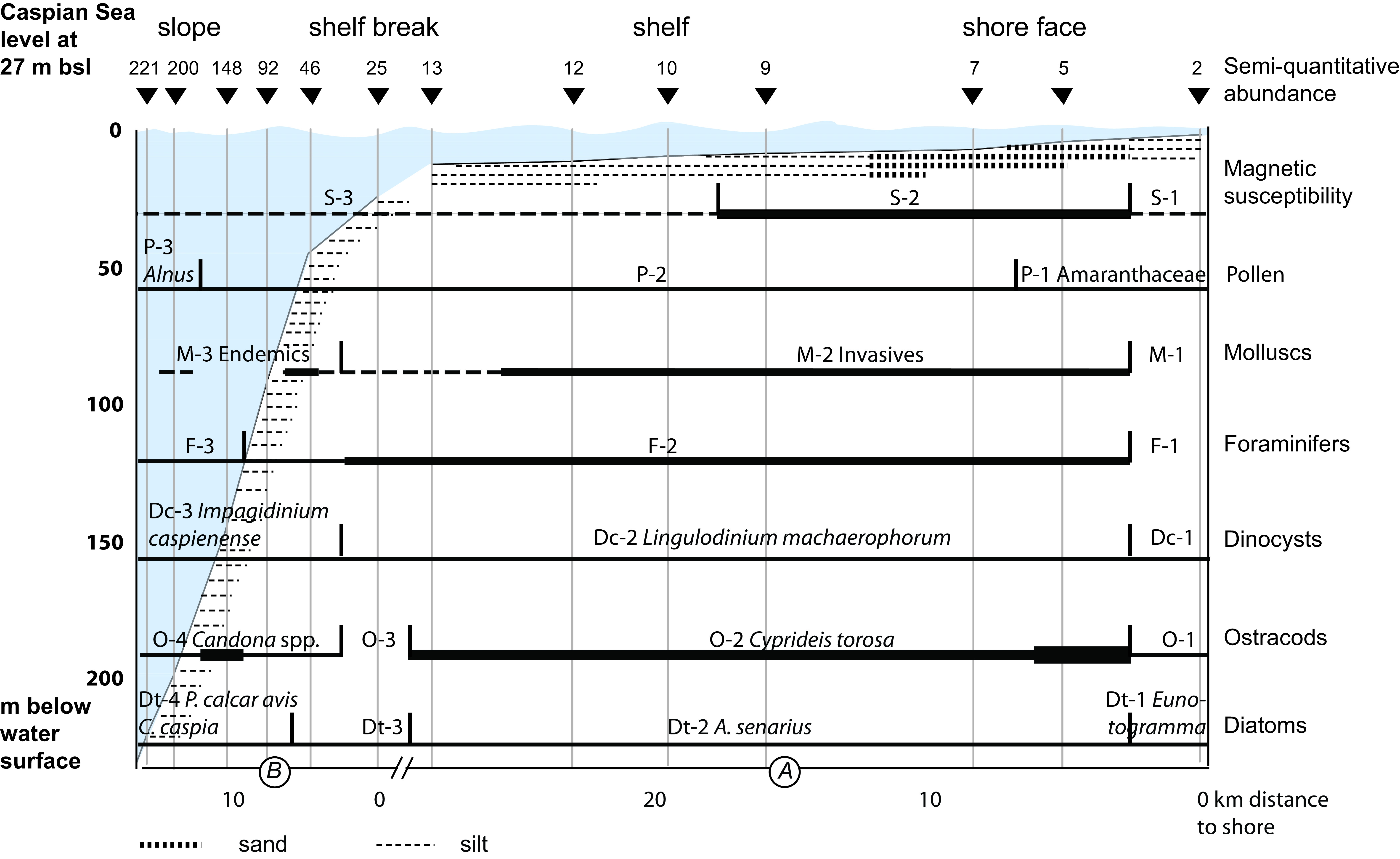
138Figure 10. Synthetic profile. Lithology only for the sediment surface. Thickness of line as an indication of proxy abundance. Horizontal distance corresponds to distance travelled by boat.

139Further out, wave action picks up, as well as coastal currents, and sands are deposited between 5 and 7 m. The maximal total absolute abundance of ostracods and high abundance of foraminifers at 5 m corresponds to the sample with sand, because of concentration by winnowing. The peak of Cyprideis torosa and Tyrrhenocythere spp. reflect the higher salinities of this site.

140Shelf zone, 9 – 25 m

141This zone is dominated by silt and is rich in biota. The shelf is characterised by the dominance of the dinocyst L. machaerophorum, the ostracod C. torosa, invasive molluscs, the presence of the diatom A. senarius, and the maximal abundance of foraminifer tests (Fig. 10).

142Shelf break, 25 – 46 m

143A shelf break is observed at 25 m (Fig. 10). The main change in water temperature in February 2014 was at 90–85 m. The position of the thermocline and pycnocline in the southern Caspian Sea is deeper than those in the middle Caspian (Terziev, 1992). Measurements indicated a thermocline at 20–50 m in Babolsar in summer 2003 (Zaker et al., 2007), and, in the extreme cold weather of 2007, it reached down to 100–140 m off Anzali (Ghaffari et al., 2010).

144Slope, 46 – >221 m

145This zone is sedimentologically not different than the previous one; but the sediment is overall poorer in biota. Endemic species of molluscs dominate at 46 m corresponding to waters characterised by high winter temperature (Fig. 10). Further down the slope the dinocyst I. caspienense, the presence of the diatoms P. calcaravis and C. caspia, sparse foraminifers, the ostracod Candona sp., and the absence of molluscs are observed.

146Depths greater than the current transect

147Based on published accounts, it is also possible to predict how changes will occur at greater depths for the biological proxies. Some information is available for the southern basin from Gofman (1966), Yassini (1986)andLeroy et al. (2007, 2013c) and for the middle basin from Boomer et al. (2005) and Leroy et al. (2007, 2014). In the deepest parts, pollen and dinocysts are present in similar abundance (e.g. core GS05 ~518 m water depth, Leroy et al., 2013c). In pilot core CP04 (associated with core GS05, Leroy et al., 2007), diatoms are present in the upper sediments. Marine to brackish species (Actinocyclus ehrenbergii, Grammatophora oceanica and Coscinodiscus argus) dominate the poorly-diversified and poorly-preserved assemblages (Chalié et al., unpublished). Foraminifers are completely absent. Using Gofman’s data, Yassini (1986) noted that ostracods were present in samples to depths of 880 m in the southern basin but Gofman (1966) regarded those below 700 m as transported. Boomer et al. (2005) and unpublished work by one of us on Holocene sediments in the Caspian Sea confirm that ostracods are present often in great numbers at considerable depths although whether they truly dwelt there is not known. Molluscs live in very low numbers all the way to the deepest parts of the Caspian Basin (Zhadin, 1965).

148Transect break

149It is also clear from our data that the transect break from part A to part B between 13 and 25 m does not directly correspond to where changes in the biotic assemblages take place. If one ignores the very shallow part of the transect (2–5 m) influenced by the Gorgan River, the main changes in the transect occur for the sedimentological data (grain size and MS) at 9–10 m, the ostracods at 25 m, then simultaneously diatoms, molluscs and dinocysts at 25–46 m, and finally foraminifers at 92–148 m (although their abundance declines already below 25 m). Pollen spectra change at 148–200 m. Therefore, various proxies have different sensitivities (such as lags, thresholds and seasonality) to the same environmental change and hence are complementary. Moreover a relative homogeneity of the shelf emerges from our data. This is supported by more general and less local studies of the south Caspian basin (Lahijani et al., accepted) and of the Turkmenistan shelf from Soviet literature (Klenova et al. 1962). This relative homogeneity is however occasionally disrupted by mud volcanoes.

6.3. Reworked biota and downslope transport

150Reworked pollen and spores amount to a median of 2% (of terrestrial pollen) with one maximum of 7% at 200 m. In the plankton, reworked dinocysts are always lower than 1%. These values are low and fall within the usual range for marine sediment. No obvious sign of reworking has been noted in the diatoms, but many of them are planktonic species, and all sites record assemblages composed of tolerant freshwater, brackish and marine species in various proportions. Reworking is therefore possibly not visible, even if it does exist.

151The foraminifers (benthic species only) below 25 m found with absolute abundances of 20–30 per g are all clearly transported. Furthermore, at some deep stations, ostracod assemblages contain shallow dwelling taxa and there are rare occurrences of charophytes that originated in coastal lagoons. Nevertheless very few ostracods could positively be identified as being reworked from much older sediments. The molluscs contain a significant number of abraded individuals that were counted separately, but molluscs were scarce below 92 m. The specimens found at the greater transect depths did not show signs of reworking. These observations of the biota fit well with the remarks made on the isotopic trends, especially the lower δ¹⁸O values for the foraminifers. Tephra morphology shows clear signs of reworking but that could have been due to aeolian remobilisation or run-off from the catchment. No volcanic eruptions are currently taking place in the area.

152Overall a small but significant proportion of the fauna/flora, especially amongst the benthic biota or proxies, show evident signs of reworking. It is likely that more specimens have been transported but without showing any physical signature. It is important to note that it remains difficult to establish objective criteria to define a reworked appearance for many different biota and researchers working on Quaternary sequences should take this into consideration.

153For the explanation of the presence of reworked fossils, two hypotheses must be examined. The first is downslope transport. High waves with a return period of 50 years could reach up to 14 m height in the east of the south Caspian Sea (Terziev, 1992), but would not reach the coast itself. Strong storm waves and wave-induced currents could nevertheless rework the upper shelf surface sediments in an event-like fashion. In the deeper parts, fast currents attributed to long waves are strong enough to transport fine sands, and the shells of microorganisms, to deeper parts (Bondarenko, 1994; Ghaffari & Chegini, 2010).

154The second hypothesis concerns in-situ vertical reworking by bioturbation. Indeed in the Caspian Sea, frequent water-level changes may move upwards, and bring for example, older sediment into the wave-breaking zone. However the sedimentation rate along the south coast of Iran is relatively high: in the Gorgan Bay it is between 1.4 and 2.4 mm/year (Karbassi & Amirnezhad, 2004); in the upper shelf it changes to 20 mm/year off Anzali (Leroy et. al., 2013b), to 9 and 14 mm/year in the west and east of Sefidrud river respectively (Vahabi Moghadam et al., 2006), and 9 mm/year off Langarud (Sharmad et al., 2012). Furthermore, coarse sediment has only been found at the depths of 5–7 m along the transect; this clearly excludes winnowing and concentration of older shells elsewhere. These observations are in favour of hypothesis one, hence downslope transport is the main reworking mechanism at present. Hence this indicates that currents are more important than previously suggested for a very shallow and wide shelf.

6.4. Presence of endemics and invasive species

155All biota examined in this investigation have endemic forms, species or even genera typical for the Caspian region. In the pollen assemblages, Parrotia persica (DC.) C.A.Mey, the Persian ironwood, a member of the Hamamelidaceae, has its distribution only in the northern slopes of the Alborz Mountains up to 1500 m elevation. It was present in Europe during large part of the Quaternary but disappeared at a currently undetermined time (Leroy & Roiron, 1996). Among the dinocysts, Caspidinium, a genus recently described, is found in the Caspian Sea and also in the Black Sea (Marret et al., 2004, 2009). I. caspienense, a species typical of the Caspian Sea, is currently very abundant, often dominant. It has been the case since 4 ka ago when the salinity of the Caspian Sea changed from slightly brackish (~7 psu) (possibly 5–7 psu) to the present 13 psu (Leroy et al., 2013a, 2013c, 2014). Its ecology is not well known and this transect, where it occurs in nearly all samples, confirms tolerance of salinities of ~12 psu and winter surface temperature of 6.5–11.5 °C. Although far from being endemic species, L. machaerophorum displays cyst forms typical of low salinity environments (Mertens et al., 2009) and shows a clear increase in the last few decades (Leroy et al., 2013b). Among the identified diatomspecies, T. caspica is the only clearly endemic one to the Caspian Sea. Perhaps also some other rare and unidentified species of Thalassiosira exist. Most other species that thrive are either known for euryhalinity or to behave as such, in the particular context of the strongly variable salinity conditions of the Caspian Sea. This relative large number of endemic species in most groups necessitates detailed taxonomic study in order to avoid confusion by the Quaternary scientific community.

156The invasive diatom species Pseudosolenia calcar avis (Karpevitch, 1975 in Karpinsky, 2010) that most likely penetrated in the Caspian Sea from the Black Sea, was observed for the first time in the southern Caspian Sea basin in 1934 (as a Rhizosolenia species). The invasion started from Astrabadsky Bay (Gorgan Bay), just parallel to and south of the present transect. After a period when P. calcar avis reached a very high biomass, established a competitive edge and dominated the phytoplankton community in most areas of the middle and southern Caspian Sea basins, the species declined in the early 2000s (Karpinsky, 2010). It is now present in the whole Caspian Sea, but no longer dominant as an indirect consequence of the invasion of the comb jelly Mnemiopsis leidyi. In this study P. calcar avis was found in the deeper part of the Gorgan transect from 46 m, downwards and was the most abundant, or even dominant species, in the assemblages at sites from 92 and 148 m water-depth. Apart from Cyprideis torosa that has a wide distribution in the northern hemisphere, all of the ostracods identified have their origins in the Pontocaspian region and are not therefore regarded as “invasive”. Invasive mollusc species dominate the shelf and shallow slope down to 46 m. The apparent peak of seemingly fresh endemics at 46 m deserves further study.

157In the Caspian Sea, it seems that i) planktonic forms have disappeared (e.g. foraminifers and ostracods), and that ii) biota groups contain species that are very euryhaline, or even more euryhaline in the Pontocaspian than in the rest of their distribution (e.g. diatoms). This flexibility regarding ecological conditions makes many species ideal candidates for becoming successful invasive species in lakes and seas worldwide.

6.5. Dating

158Radiocarbon dating of samples from the Caspian Sea is complicated by the reservoir effect. A summary of reservoir effect estimations is given in Leroy et al. (2011) and Naderi Beni et al. (2013). However both spatial and temporal changes in the effect are likely. The current study has clearly shown the presence of tephra horizons in the sediment cores. This indicates good potential to establish the extent of reservoir effects and offsets of mollusc or ostracods at the same levels, if those tephras can be dated by geochemical correlation to eruptions of known age, or through ¹⁴C dating of associated material in terrestrial contexts. Realistically, we may find only tephra from the Caucasus/Iran, where the eruptive history, especially for the Holocene is poorly known. Given the absence of comparative glass data from these sources, we may not be able to say which volcano contributed the ash unless samples from the volcanoes can be obtained. However, the source of the tephra need not be known to use geochemically-distinctive tephras as a means of correlating and dating terrestrial, lacustrine and marine cores. Identification of more distal, and thus sparser, tephras (e.g. from the Mediterranean region) could be complicated if the background of detrital tephra is strong. Further investigations of a sedimentary sequence are required to evaluate the full potential of this technique.

6.6. The basis for a calibration of proxies

159At the scale of the last glacial-interglacial cycle, water levels have fluctuated very rapidly, but the chronology and the amplitude (up to ~150 m vertical amplitude) of these changes are poorly known. The water level history has mostly been reconstructed from outcrops where low levels are recorded by sedimentary hiatus (Leroy et al., 2013a and references therein). With the developing coring capacity in the Caspian Sea, it has become possible to take some sediment cores offshore spanning >15,000 years for scientific purposes (Levchenko & Roslyakov, 2010; Leroy et al., 2013a, 2014)and hence obtain continuous proxy records of past changes. Multi-proxy studies such as the present one, when repeated in other parts of the Pontocaspian region with other oceanographic characteristics, will benefit semi-quantitative and quantitative palaeoenvironmental reconstructions.

160For the dinocysts, a previous publication suggested that the abundance of L. machaerophorum was not linked to salinity but to temperature (Leroy et al., 2013b). Here it can be added that shallow water depths are favourable to this species due to lower temperature inertia.

161One of the distinguishing features of the present-day Caspian Sea diatom flora is an extremely wide euryhalinity of species, in particular marine species, as compared to seas (Karayeva & Makarova, 1973). Indeed, most of the marine species that are present in the Caspian Sea adapted well even to the lower salinity basin in the northern Caspian Sea (Proshkina-Lavrenko & Makarova, 1968; Genkal, 1992). Diatom assemblages show variations in composition along the studied transect. Because of fairly constant salinity and temperature, driving factors of the diatom distribution is probably related to something other than these two parameters. Depth as such can hardly be invoked as a major forcing factor, as surface sediment contains diatoms that are photosynthetic and once lived in the surface waters, irrespective of the depth of the site. A seasonal hydrochemical survey would also be necessary to determine the forcing factor.

162Some ostracod species have a clear depth distribution in this study. In particular C. torosa, T. amnicola and T. azerbaijanica inhabit depths of 13 m or less whereas Candona spp. and E. naphtatscholana were found only at and below 46 m. Whether this is due to temperature, salinity, substrate or some other factor is not known yet. For the molluscs, building on the Kosarev & Yablonskaya (1994) review, the present study provides environmental parameters in the same station as the biotic samples.

163A plausibility test for the oxygen isotope composition in the different taxonomic groups may clarify their specific potential as palaeoproxies for use in core sediments, such as measurements on multiple specimens in each sample and analyses on the range of values. High-resolution isotopic studies such as those of Vonhof et al. (2004) on mollusc shells a few millennia old have started to provide an insight into seasonality.

7. Conclusions

164Our investigations present the results of a unique multidisciplinary study of oceanographical, sedimentological and biological data from thirteen disciplines, some of them never studied before in a surface transect in the Caspian Sea, e.g. dinocysts, diatoms and tephras. Thirteen sediment samples were taken along a near continuous depth transect from the coast to 221 m in the SE corner of the Caspian Sea, which is the warmest of the Pontocaspian region. The main variables were depth (especially for benthic biota) and shore proximity; temperature and especially salinity variations are minimal. Future studies should be made along transects of varying salinity or temperature to complement the present work.

165On one hand the Gorgan transect represents a baseline as of 2014 for any comparison to the past and to the future. The region is expected to change as it becomes more densely populated and industrialised, and the region is also not spared from climatic change, experiencing a dramatic drop of 1 m between 1995 and 2005. On the other hand, the current study lays the foundation for a calibration of these biotic assemblages, often dominated by endemic species, for future Quaternary palaeoecological studies. The main results are a finer differentiation of the shore face (2–7 m), shelf (9–25 m) and slope (46–>221 m) by biota than by sedimentology. The current study indicates that radiocarbon dating Caspian Sea sediment is still a challenge; but a potential to develop tephrostratigraphy exists. Amongst the diverse biotic groups examined, molluscs exhibited the highest rate of invasion by far. Endemism was marked in most groups, but least so in the diatoms and ostracods. Many biota have forms adapted to low salinities.

166Stable oxygen isotopes measured in ostracod tests enabled us to faithfully reconstruct present-day water temperatures along the water column; hence ostracods are plausibly well-suited for the reconstruction of past water temperatures. Foraminifers and molluscs did not reflect the water temperature profile as expected and may not be suitable for such an approach in the Caspian Sea.

167A clear caveat for the uncritical use of surface transect data for the creation of calibration sets is the occurrence of reworked biota and transport from the shallow depths to the deep ones, even in areas of relative wide shelf. Any further studies can address this by staining living specimens in the field. A new international project (Marie S. Curie PRIDE Pontocaspian biodiversity rise and demise) has already included the present approach in its programme.

8. Acknowledgments

168We are indebted to Brunel University London (BUL) for an award from the Research Development Fund that covered expenses fieldwork, palynological extraction work and four radiocarbon dates. We are grateful to the PRIDE project that has received funding from the European Union's Horizon 2020 research and innovation programme under the Marie Sklodowska-Curie grant agreement No 642973.

169Mr Mortazavi, the head of the Department of the Environment station in Bandar-e-Torkman, generously provided the use of the inflatable boat for Part A of the transect. Sean Pyne-O’Donnell kindly assisted with the tephra preparations. James Davy of the Earth Sciences Department at University College London is thanked for providing the SEM images of ostracods. We are grateful to Jean-Charles Mazur for water content and diatom samples preparation at the CEREGE. We are grateful to M. Sala, L. López-Merino and T. Hoyle (BUL), who critically read an earlier version of this paper, and to the reviewers. NASA Ocean Biology (OB.DAAC) is acknowledged for preparing the MODIS Chl-a and SST data.

170The data have been contributed to the Neotoma database.

9. References

171Agalarova, D.A., Kadyrova, Z.K. & Kulieva, S.A., 1961. Ostracoda from the Pliocene and post-Pliocene deposits of Azerbaijan. Azerbaijan State Publisher, Baku, 420 p. [In Russian].

172Albrecht, C. & Wilke, T., 2008. Ancient Lake Ohrid: biodiversity and evolution. Hydrobiologia, 615, 103–140. https://doi.org/10.1007/s10750-008-9558-y

173Arpe, K. & Leroy, S.A.G., 2007. The Caspian Sea Level forced by the atmospheric circulation, as observed and modelled. Quaternary International, 173-174, 144–152. https://doi.org/10.1016/j.quaint.2007.03.008   

174Arpe, K., Bengtsson, L., Golitsyn, G.S., Mokhov, I.I., Semenov, V.A. & Sporyshev, P.V., 2000. Connection between Caspian Sea level variability and ENSO. Geophysical Research Letters, 27/17, 2693–2696. https://doi.org/10.1029/1999GL002374

175Arpe, K., Leroy, S.A.G., Lahijani, H. & Khan, V., 2012. Impact of the European Russia drought in 2010 on the Caspian Sea level. Hydrology and Earth System Science, 16, 19–27. https://doi.org/10.5194/hess-16-19-2012

176Arpe, K., Leroy, S.A.G., Wetterhall, F., Khan, V., Hagemann, S. & Lahijani, H., 2014. Prediction of the Caspian Sea Level using ECMWF seasonal forecast and reanalysis. Theoretical and Applied Climatology, 117, 41–60. https://doi.org/10.1007/s00704-013-0937-6

177Athersuch, J., 1979. The ecology and distribution of the littoral ostracods of Cyprus. Journal of Natural History, 13, 135–160. https://doi.org/10.1080/00222937900770111a

178Athersuch, J., Horne, D.J. & Whittaker, J.E., 1989. Marine and brackish water ostracods. E.J. Brill for the Linnean Society of London, Leiden, Synopsis of the British Fauna (New Series), 43. 343 p.

179Bagheri, S., Mansor, M., Turkoglu, M., Makaremi, M. & Babaei, H., 2012. Temporal distribution of phytoplankton in the South-western Caspian Sea during 2009–2010: a comparison with previous surveys. Journal of the Marine Biological Association of the United Kingdom, 92/6, 1243–1255.https://doi.org/10.1017/S0025315412000094

180Bastami, K.D., Taheri, M., Bagheri, H., Foshtomi, M.Y., Ganji, S., Haghparast, S., Soltani, F., Hamzehpoor, A. & Karimi, B., 2014. Response of sediment-dwelling annelida community in relation to geochemical parameters in the Gorgan Bay, Caspian Sea. International Journal of Environmental Science and Technology, 11, 2025–2036. https://doi.org/10.1007/s13762-014-0658-0

181Bengston, P., 1988. Open nomenclature. Palaeontology, 31/1, 223–227.

182Bennett, K., 2007. Psimpoll and Pscomb Programs for Plotting and Analysis. Version Psimpoll 4.27. http://chrono.qub.ac.uk/psimpoll/psimpoll.html, last accessed on 11 December 2015.

183Birks, H.J.B., 2003. Quantitative palaeoenvironmental reconstructions from Holocene biological data. In Mackay, A., Battarbee, R.W., Birks, H.J.B. & Oldfield, F. (eds), Global Change in the Holocene. Arnold, London, 107–123.

184Birshtein, Y.A., Vinogradov, L.G., Kondakov, N.N., Astakhova, M.S. & Romanova, N.N. (eds), 1968. Atlas of Invertebrates of the Caspian Sea. Pishchevaya Promyshlennost, Moscow, 415 p. [In Russian].

185Bondarenko, A.L., 1993. Techeniya Kaspiiskogo morya i formirovanie polya solenosti vod Severnogo Kaspiya (Caspian Sea currents and the formation of salinity field in the Northern Caspian Sea). Moscow, Nauka, 122 p. [In Russian].

186Bondarenko, A.L., 1994. Natural investigation of the Caspian Sea currents. In Khublarian M.G. (ed.), Water of Continent: Problems and Solutions. Russian Academy of Science, Water Problems Institute, Moscow, 389–396.

187Boomer, I., von Grafenstein, U., Guichard, F. & Bieda, S., 2005. Modern and Holocene sublittoral ostracod assemblages (Crustacea) from the Caspian Sea: A unique brackish, deep-water environment. Palaeogeography, Palaeoclimatology, Palaeoecology, 225, 173–186. https://doi.org/10.1016/j.palaeo.2004.10.023

188Burchardt, B. & Fritz, P., 1980. Environmental isotopes as environmental and climatological indicators. In Fritz P. & Fontes J.C. (eds), Handbook of Environmental Isotope Geochemistry, vol. 1A. Elsevier, New York, 433–504.

189Chekhovskaya, M.P., Stepanova, A.Yu, Khusid, T.A., Matul, A.S. & Rakowski, A.Z., 2014. Late Pleistocene – Holocene Ostracod Assemblages of the Northern Caspian Sea Shelf. Oceanology, 54/2, 212–221 (Translated from Russian by Pleiades Publishing Inc., 2014). https://doi.org/10.1134/S0001437014020040

190Davidson, J., Hassanzadeh, J., Berzins, R., Stockli, D.F., Bashukooh, B., Turrin, B. & Pandamouz, A., 2004. The geology of Damavand volcano, Alborz Mountains, northern Iran. Bulletin of the Geological Society of America, 116/1-2, 16–29. https://doi.org/10.1130/B25344.1

191Dumont, H.J., 1998. The Caspian Lake: History, biota, structure, and function. Limnology and Oceanography, 43/1, 44–52. https://doi.org/10.4319/lo.1998.43.1.0044

192ECMWF, 2015. European Centre for Medium-Range Weather Forecasts, ERA-interim. http://apps.ecmwf.int/datasets, last accessed on 2 October 2018.

193Epstein, S., Buchsbaum, R., Lowenstam, H.A. & Urey, H.C., 1953. Revised carbonate-water isotopic temperature scale. Bulletin of the Geological Society of America, 64, 1315–1326. https://doi.org/10.1130/0016-7606(1953)64[1315:RCITS]2.0.CO;2

194Etiope, G., 2005. Mud volcanoes and microseepage: the forgotten geophysical component of atmospheric methane budget. Annals of Geophysics, 48, 1, 1–7. https://doi.org/10.4401/ag-3175

195Forte, A.M. & Cowgill, E., 2013. Late Cenozoic base-level variations of the Caspian Sea: a review of its history and proposed driving mechanisms. Palaeogeography, Palaeoclimatology, Palaeoecology, 386, 392–407. https://doi.org/10.1016/j.palaeo.2013.05.035

196Froehlich, K., 2000. Evaluating the water balance of inland seas using isotopic tracers: the Caspian Sea experience. Hydrological Processes, 14, 1371–1383. https://doi.org/10.1002/1099-1085(20000615)14:8<1371::AID-HYP141>3.0.CO;2-T

197Froehlich, K., Rozanski, K., Povinec, P., Oregioni, B. & Gastaud, J., 1999. Isotope studies in the Caspian Sea. Science of the Total Environment, 237-238, 419–427. https://doi.org/10.1016/S0048-9697(99)00154-0

198Gasanova, A.S., Guseynov, K.M. & Guseynov, M.K., 2014. Phytoplankton species composition of the Russian sector of the Caspian Sea. Ecology of Plants. The South of Russia: ecology, development, 9/2, 102–108. https://doi.org/10.18470/1992-1098-2014-2-102-108. [In Russian].

199Gatti, E., Saidin, M., Talib, K., Rashidi, N., Gibbard, P. & Oppenheimer, C., 2013. Depositional processes of reworked tephra from the Late Pleistocene Youngest Toba Tuff deposits in the Lenggong Valley, Malaysia. Quaternary Research, 79, 228–241. https://doi.org/10.1016/j.yqres.2012.11.006

200Genkal, S.I., 1992. Atlas of the diatom algae of the plankton in the Volga river. Gidrometeoizdat, St.-Petersburg, 128 p. [In Russian].

201Ghaffari, P. & Chegini, V., 2010. Acoustic Doppler Current Profiler observations in the southern Caspian Sea: shelf currents and flow field off Feridoonkenar Bay, Iran. Ocean Science, 6, 737–748.https://doi.org/10.5194/os-6-737-2010

202Ghaffari, P., Lahijani, H.A.K. & Azizpour, J., 2010. Snapshot observation of the physical structure and stratification in deep-water of the South Caspian Sea (western part). Ocean Science, 6, 877–885. https://doi.org/10.5194/osd-6-2555-2009

203Ghane, F., Sadough, M., Manouchehri, H., Moghaddasi, B. & Hasankiadeh, N.M., 2014. Identification and abundance of benthic foraminifera in sediments of Southern Caspian Sea from Bahnamir to Babolsar, Iran. International Journal of Marine Science, 4, 11, 99–107. https://doi.org/10.5376/ijms.2014.04.0011

204Gilg, H.A., Struck, U., Vennemann, T. & Boni, M., 2003. Phosphoric acid fractionation factors for smithsonite and cerussite between 25 and 72°C. Geochimica et Cosmochimica Acta, 67/21, 4049–4055. https://doi.org/10.1016/S0016-7037(03)00169-8

205Global Volcanism Programme, 2013. Elbrus. Kazbek. https://volcano.si.edu/volcano.cfm?vn=214010. https://volcano.si.edu/volcano.cfm?vn=214020, last accessed on 3 October 2018.

206Gofman, E.A., 1966. Ecology of modern and Novocaspian ostracods of the Caspian Sea. Akademie NAUK, SSSR, Moscow, 183 p. [In Russian].

207Grigorovitch, I.A., Therriault, T.W. & MacIsaac, H.J., 2003. History of aquatic invertebrate invasions in the Caspian Sea. Biological Invasions, 5, 103–115. https://doi.org/10.1023/A:1024050824073

208Grimm, E., 1987. CONISS: a FORTRAN 77 program for stratigraphically constrained cluster analysis by the method of incremental sum of squares. Computers & Geosciences, 13/1, 13–35. https://doi.org/10.1016/0098-3004(87)90022-7

209Guiry, M.D. & Guiry, G.M., 2016. Algaebase. World-wide electronic publication, National University of Ireland, Galway. http://www.algaebase.org/, last accessed on 18 January 2016.

210Habibi, P., 2013. Distribution, diversity and morphology of Holocene benthic foraminifera assemblage of the Golestan coast. Unpublished MSc thesis, Payam Noor University, Tehran. [In Persian].

211Habibi, P., Babazadeh, A., Lahijani, H.A.K. & Abasiyan, H., 2013. Benthic foraminifera abundance of sedimentary sequence in Gorgan Bay, North of Iran. Oceanography, 15, 59–69. [In Persian].

212Haghani, S., Leroy, S.A.G., Khdir, S., Kabiri, K., Naderi Beni, M. & Lahijani, H.A.K., 2016. An early Little Ice Age brackish water invasion along the coast of the Caspian Sea (sediment of Langarud wetland) and its wider impacts on the environment and people. Holocene, 26, 1, 3–16. https://doi.org/10.1177/0959683615596835

213Hall, V.A. & Pilcher, J.R., 2002. Late-Quaternary Icelandic tephras in Ireland and Great Britain: detection, characterization and usefulness. Holocene, 12, 223–230. https://doi.org/10.1191/0959683602hl538rr

214Heiri, O., Lotter, A.F. & Lemcke, G., 2001. Loss on ignition as a method for estimating organic and carbonate content in sediments: reproducibility and comparability of results. Journal of Paleolimnology, 25, 101–110. https://doi.org/10.1023/A:1008119611481

215Hermelin, J.O. & Shimmield, G.B., 1990. The importance of the oxygen minimum zone and sediment geochemistry in the distribution of Recent benthic foraminifera in the Northwest Indian Ocean. Marine Geology,91, 1–29. https://doi.org/10.1016/0025-3227(90)90130-C

216Hoogendoorn, R.M., Boels, J.F., Kroonenberg, S.B., Simmons, M.D., Aliyeva, E., Babazadeh, A.D. & Huseynov, D., 2005. Development of the Kura delta, Azerbaijan; a record of Holocene Caspian Sea-level changes. Marine Geology, 222-223, 359–380. https://doi.org/10.1016/j.margeo.2005.06.007

217Ibrayev, R.A., Özsoy, E., Schrum, C. & Sur, H.İ., 2010. Seasonal variability of the Caspian Sea three-dimensional circulation, sea level and air-sea interaction. Ocean Science, 6, 311–329. https://doi.org/10.5194/os-6-311-2010

218Imboden, D.M. & Wuest, A., 1995. Mixing mechanisms in lakes. In Lerman, A., Imboden, D.M. & Gat, J.R. (eds), Physics and Chemistry of Lakes. Berlin, Springer-Verlag, 83–138.

219Kakroodi, A.A., Leroy, S.A.G., Kroonenberg, S.B., Lahijani, H.A.K., Alimohammadian, H., Boomer, I. & Goorabi, A., 2015. Late Pleistocene and Holocene sea-level change and coastal palaeoenvironment along the Iranian Caspian shore. Marine Geology, 361, 111–125. https://doi.org/10.1016/j.margeo.2014.12.007

220Karakhanian, A., Jrbashyan, R., Trifonov, V., Philip, H., Arakelian, S., Avagyan, A., Baghdassaryan, H., Davtian, V. & Ghoukassyan, Yu., 2003. Volcanic hazards in the region of the Armenian Nuclear Power Plant. Journal of Volcanological and Geothermal Research, 126/1-2, 31–62. https://doi.org/10.1016/S0377-0273(03)00115-X

221Karayeva, N.I. & Makarova, I.V., 1973. Specific features and origin of the Caspian Sea flora. Marine Biology, 21, 269–275.

222Karbassi, A.R. & Amirnezhad, R., 2004. Geochemistry of heavy metals and sedimentation rate in a bay adjacent to the Caspian Sea. International Journal of Environmental Science and Technology, 1/3, 191–198. https://doi.org/10.1007/BF03325832

223Karpinsky, M.G., 2005a. Biodiversity. In Kostianoy, A. & Kosarev, A. (eds), The Caspian Sea Environment. Springer, Berlin, Handbook of Environmental Chemistry, 5P, 159–173. https://doi.org/10.1007/698_5_008

224Karpinsky, M.G., 2005b. Introduced species. In Kostianoy, A. & Kosarev, A. (eds), The Caspian Sea Environment. Springer, Berlin, Handbook of Environmental Chemistry, 5P, 175–190. https://doi.org/10.1007/698_5_009

225Karpinsky, M.G., 2010. Pseudosolenia calcar-avis (Bacillariophyta, Centrophyceae) in the Caspian Sea. Russian Journal of Biological Invasions, 1/2, 81–86. https://doi.org/10.1134/S2075111710020050

226Keaveney, E.M. & Reimer, P.J. 2012. Understanding the variability in freshwater radiocarbon reservoir offsets: a cautionary tale. Journal of Archaeological Science, 39, 1306–1316. https://doi.org/10.1016/j.jas.2011.12.025

227Klenova, M.V., Solovev, V.F., Aleksina, F.A., Vikhrenko, I.M., Kulakova, L.C., Maev, E.G., Rikhter, V.G., Skorhiakova, N.S., 1962. Geological Structure of the Caspian Sea Shelf and Slope. Soviet Academy of Science, Moscow, 638 p. [In Russian].

228Kolesnikov, V.P., 1947. Key to Caspian gastropods. Byulleten Moskovsgoko Obshchestva Ispyatelei Prirody, Otdel Geologii, 22, 1–259. [In Russian].

229Komar, P.D., 1998. Beach Processes and Sedimentation, 2^nd ed. Simon and Schuster, Upper Saddle River, N. J., 544 p.

230Kosarev, A.N. & Yablonskaya, E.A., 1994. The Caspian Sea. SPB Academic Publishing, The Hague, 259 p.

231Kostianoy, A. & Kosarev, A., 2005. The Caspian Sea environment. Springer, Berlin, Handbook of Environmental Chemistry, 5P, 271 p. https://doi.org/10.1007/b138238

232Kouraev, A.V., Crétaux, J.-F., Lebedev, S.A., Kostianoy, A.G., Ginzburg, A.I., Sheremet, N.A., Mamedov, R., Zakharova, E.A., Roblou, L., Lyard, F., Calmant, S. & Bergé-Nguyen, M., 2011. Satellite altimetry applications in the Caspian Sea. In Vignudelli, S., Kostianoy, A.G., Cipollini, P. & Benveniste, J. (eds), Coastal Altimetry. Springer, Berlin, 331–366. https://doi.org/10.1007/978-3-642-12796-0_13

233Krammer, K. & Lange-Bertalot, H. (eds), 1986. Bacillariophyceae. 1. Teil, Naviculaceae. Süsswasserflora von Mitteleuropa, 2/1. Gustav Fischer, Stuttgart, 876 p.

234Krammer, K. & Lange-Bertalot, H. (eds), 1988. Bacillariophyceae. 2. Teil, Bacillariaceae, Epithemiaceae, Surirrellaceae. Süsswasserflora von Mitteleuropa, 2/2. Gustav Fischer Verlag, Stuttgart, 576 p.

235Krammer, K. & Lange-Bertalot, H. (eds), 1991a. Bacillariophyceae. 3. Teil, Centrales, Fragilariaceae, Eunotiaceae. Süsswasserflora von Mitteleuropa, 2/3. Gustav Fischer Verlag, Stuttgart, 596 p.

236Krammer, K. & Lange-Bertalot, H. (eds), 1991b. Bacillariophyceae. 4. Teil, Achnanthaceae, kritische ergänzungen zu Navicula (Lineolatae) und Gomphonema Gesamliteraturverzeichnis. Süsswasserflora von Mitteleuropa, 2/4. Gustav Fischer Verlag, Stuttgart, 437 p.

237Kroonenberg, S.B., Abdurakhmanov, G.M., Badyukova, E.N., Borg, K.V.D., Kalashnikov, A., Kasimov, N.S., Rychagov, G.I., Svitoch, A.A., Vonhof, H.B. & Wesselingh, F.P., 2007. Solar-forced 2600 BP and Little Ice Age highstands of the Caspian Sea. Quaternary International, 173, 137–143. https://doi.org/10.1016/j.quaint.2007.03.010

238Lahijani, H., Tavakoli, V. & Hosseindoost, M., 2007. History of Caspian environmental changes by molluscan isotope records. Journal of Coastal Research, SI 50, 438 – 442.

239Lahijani, H., Tavakoli, V. & Amini, A., 2008. River mouth configuration in South Caspian Coast, Iran. Environmental Sciences, 5/2, 65–86.

240Lahijani, H.A.K., Rahimpour-Bonab, H., Tavakoli, V. & Hosseindoost, M., 2009. Evidence for Late Holocene high-stands in Central Gilān–East Mazanderan, South Caspian coast, Iran. Quaternary International, 197, 55–71. https://doi.org/10.1016/j.quaint.2007.10.005

241Lahijani, H., Abbasian, H., Naderi–Beni, A., Leroy, S.A.G., Haghani, S., Habibi, P., Hosseindust, M., Shahkarami, S., Yeganeh, S., Zandi, Z., Tavakoli, V., Azizpour, J., Sayed-Valizadeh, M., Pourkerman, M., Shah-Hosseini, M. Accepted March 2018 Distribution pattern of South Caspian Sea sediment. Canadian Journal of Earth Sciences.  https://doi.org/10.1139/cjes-2017-0239

242Leroy, S.A.G. & Roiron, P., 1996. Final Pliocene macro and micro floras of the paleovalley of Bernasso (Escandorgue, France). Review of Palaebotany and Palynology, 94, 295–328. https://doi.org/10.1016/S0034-6667(96)00016-4

243Leroy, S.A.G., Marret, F., Giralt, S. & Bulatov, S.A., 2006. Natural and anthropogenic rapid changes in the Kara-Bogaz Gol over the last two centuries by palynological analyses. Quaternary International, 150, 52–70. https://doi.org/10.1016/j.quaint.2006.01.007

Leroy, S.A.G., Marret, F., Gibert, E., Chalié, F., Reyss, J.-L. & Arpe, K., 2007. River inflow and salinity changes in the Caspian Sea during the last 5500 years. Quaternary Science Reviews, 26, 3359–3383.https://doi.org/10.1016/j.quascirev.2007.09.012

244Leroy, S.A.G., Lahijani, H.A.K., Djamali, M., Naqinezhad, A., Moghadam, M.V., Arpe, K., Shah-Hosseini, M., Hosseindoust, M., Miller, Ch.S., Tavakoli, V., Habibi, P. & Naderi Beni, M., 2011. Late Little Ice Age palaeoenvironmental records from the Anzali and Amirkola lagoons (south Caspian Sea): vegetation and sea level changes. Palaeogeography, Palaeoclimatology, Palaeoecology, 302, 415–434. https://doi.org/10.1016/j.palaeo.2011.02.002

245Leroy, S.A.G., Kakroodi, A.A., Kroonenberg, S.B. & Lahijani, H.A.K., Alimohammadian, H., Nigarov, A., 2013a. Holocene vegetation history and sea level changes in the SE corner of the Caspian Sea: relevance to SW Asia climate. Quaternary Science Reviews, 70, 28–47. https://doi.org/10.1016/j.quascirev.2013.03.004

246Leroy, S.A.G., Lahijani, H.A.K., Reyss, J.-L., Chalié, F., Haghani, S., Shah-Hosseini, M., Shahkarami, S., Tudryn, A., Arpe, K., Habibi, P., Nasrollahzadeh, H.S. & Makhlough, A., 2013b. A two-step expansion of the dinocyst Lingulodinium machaerophorum in the Caspian Sea: the role of changing environment. Quaternary Science Reviews, 77, 31–45. https://doi.org/10.1016/j.quascirev.2013.06.026

247Leroy, S.A.G., Tudryn, A., Chalié, F., López-Merino, L. & Gasse, F., 2013c. From the Allerød to the mid-Holocene: palynological evidence from the south basin of the Caspian Sea.Quaternary Science Reviews, 78, 77–97. https://doi.org/10.1016/j.quascirev.2013.07.032

248Leroy, S.A.G., López-Merino, L., Tudryn, A., Chalié, F. & Gasse, F., 2014. Late Pleistocene and Holocene palaeoenvironments in and around the Middle Caspian Basin as reconstructed from a deep-sea core. Quaternary Science Reviews, 101, 91–110. https://doi.org/10.1016/j.quascirev.2014.07.011

249Levchenko, O.V. & Roslyakov, A.G., 2010. Cyclic sediment waves on western slope of the Caspian Sea as possible indicators of main transgressive/regressive events. Quaternary International, 225, 210–220. https://doi.org/10.1016/j.quaint.2009.12.001

250Levin, I. & Kromer, B., 2004. The tropospheric ¹⁴CO₂ level in mid-latitudes of the Northern Hemisphere (1959-2003). Radiocarbon, 46/3, 1261–1272. https://doi.org/10.2458/rc.v46i3.4181

251Levin, I., Kromer, B. & Hammer, S., 2013. Atmospheric Δ¹⁴CO₂ trend in Western European background air from 2000 to 2012. Tellus B-Chemical and Physical Meteorology, 65, 20092. https://doi.org/10.3402/tellusb.v65i0.20092

252Lewis, D.W. & McConchie, D., 1994. Analytical Sedimentology. Chapman & Hall, New York, 197 p.

253Linke, P. & Lutze, G.F., 1993. Microhabitat preferences of benthic foraminifera – a static concept or a dynamic adaptation to optimize food acquisition? Marine Micropaleontology, 20, 215–34. https://doi.org/10.1016/0377-8398(93)90034-U

254Loeblich, A.R. & Tappan, H., 1987. Foraminiferal genera and their classification. Van Nostrand Reinhold, New York, 970 p.

255Mandelstam, M., Markova, L., Rosyeva, T. & Stepanaitys, N., 1962. Ostracoda of the Pliocene and Post-Pliocene deposits of Turkmenistan. Turkmenistan Geological Institute, Ashkhabad. 288 p. [In Russian].

256Marret, F., Leroy, S., Chalié, F. & Gasse, F., 2004. New organic-walled dinoflagellate cysts from recent sediments of central Asian seas. Review of Palaeobotany and Palynology, 129, 1– 20. https://doi.org/10.1016/j.revpalbo.2003.10.002

257Marret, F., Mudie, P., Aksu, A. & Hiscott, R.N., 2009. A Holocene dinocyst record of a two-step transformation of the Neoeuxinian brackish water lake into the Black Sea. Quaternary International, 197, 1-2, 72–86. https://doi.org/10.1016/j.quaint.2007.01.010

258Matishov, G.G., Yaitskaya, N.A. & Berdnikov, S.V., 2012. Peculiarities of the centennial salinity regime of the Caspian Sea. Doklady Akademii Nauk, 444/2, 747–751. [In Russian].

259Mayer, E.M., 1972. Modern foraminifers of Preapsheron region, Caspian Sea. In Zevina, G.B. & Maev, E.G. (eds), Complex Investigation of the Caspian Sea. Moscow St. Univ., 3, 5–24.

260McCarthy, F.M.G. & Mudie, P.J., 1998. Oceanic pollen transport and pollen: dinocyst ratios as markers of late Cenozoic sea level change and sediment transport. Palaeogeography, Palaeoclimatology, Palaeoecology, 138, 187–206. https://doi.org/10.1016/S0031-0182(97)00135-1

261Mertens, K.N., Ribeiro, S., Bouimetarhan, I. …, Louwye, S., 2009. Process length variation in cysts of a dinoflagellate, Lingulodinium machaerophorum, in surface sediments: investigating its potential as salinity proxy. Marine Micropaleontology, 70, 54–69. https://doi.org/10.1016/j.marmicro.2008.10.004

262Minnett, P.J., Brown, O.B., Evans, R.H., Key, E.L., Kearns, E.J., Kilpatrick, K., Kumar, A., Maillet, K.A. & Szczodrak, G., 2004. Sea-surface temperature measurements from the moderate-resolution imaging spectroradiometer (MODIS) on aqua and terra. IEEE International Geoscience and Remote Sensing Symposium, 2004. IGARSS ’04. Proceedings. https://doi.org/10.1109/igarss.2004.1370173

263Naderi Beni, A., Lahijani, H., Harami, R.M., Arpe, K., Leroy, S.A.G., Marriner, N., Berberian, M., Andrieu-Ponel, V., Djamali, M., Mahboubi, A. & Reimer, P.J., 2013. Caspian sea-level changes during the last millennium: historical and geological evidence from the south Caspian Sea. Climate of the Past, 9/4, 1645–1665. https://doi.org/10.5194/cp-9-1645-2013

264Nasrollahzadeh, S.H., Makhlough, A., Eslami, F. & Leroy, S.A.G., 2014. Features of the phytoplankton community in the Southern Caspian Sea, a decade after the invasion of Mnemiopsis leidyi. Iranian Journal of Fisheries Sciences, 13/1, 145–167.

265Nezlin, N.P., 2005. Patterns of seasonal and interannual variability of remotely sensed Chlorophyll. In Kostianoy, A. & Kosarev, A. (eds), The Caspian Sea Environment. Springer, Berlin, Handbook Environmental Chemistry, 5P, 143–157. https://doi.org/10.1007/698_5_007

266Nordyke, M.D., 2000. The Soviet Program for Peaceful Uses of Nuclear Explosions. Lawrence Livermore National Laboratory, 1 September 2000. https://e-reports-ext.llnl.gov/pdf/238468.pdf, last accessed on 11 December 2015.

267OceanColor web (no date). http://oceancolor.gsfc.nasa.gov/cgi/browse.pl?sen=am, last accessed on 26 December 2016.

268Ojaveer, E., Leppäkoski, E., Olenin, S. & Ricciardi, A., 2002. Ecological impact of Ponto-Caspian invaders in the Baltic Sea, European inland waters and the Great Lakes: an inter-ecosystem comparison. In Leppäkoski, E., Gollasch, E. & Olenin S. (eds), Invasive Aquatic Species of Europe: distribution, impacts and management. Kluwer Academic Publishers, Dordrecht, 412–425.

269Peeters, F., Kipfer, R., Achermann, D., Hofer, M., Aeschbach-Hertig, W., Beyerle, U., Imboden, D.M., Rozanski, K. & Fröhlich, K., 2000. Analysis of deep-water exchange in the Caspian Sea based on environmental tracers. Journal of Deep-Sea Research, 1/47, 621–654.

270Peragallo, H & Peragallo, M, 1897-1908. Atlas des Diatomées marines de France et des districts maritimes voisins. M.J. Tempère, Grez-sur-Loing, 1132 p.

271Proshkina-Lavrenko, A.I. & Makarova, I.V., 1968. Plankton algae of the Caspian Sea. Nauka, Leningrad, 291 p. [in Russian].

272Rau, G.H., Riebesell, U. & WolfGladrow, D., 1997. CO_2aq-dependent photosynthetic ¹³C fractionation in the ocean: A model versus measurements. Global Biogeochemical Cycles, 11/2, 267–278.https://doi.org/10.1029/97GB00328

273Reille, M., 1992. Pollen et Spores d'Europe et d'Afrique du Nord. Laboratoire de Botanique Historique et Palynologie, CNRS, Marseille, 520 p.

274Reille, M., 1995. Pollen et spores d’Europe et d’Afrique du Nord, Supplément 1. Laboratoire de Botanique Historique et Palynologie, Marseille, 327 p.

275Reille, M., 1998. Pollen et spores d’Europe et d’Afrique du Nord, Supplément 2. Laboratoire de Botanique Historique et Palynologie, Marseille, 521 p.

276Reimer, R.W. & Reimer, P.J., 2018. CALIBomb www program. 14CHRONO Centre, Queen's University Belfast. http://calib.qub.ac.uk/CALIBomb/, last accessed 2 October 2018.

277Reimer, P.J., Baillie, M.G.L., Bard, E., Bayliss, A., Beck, J.W., Bertrand, C., Blackwell, P.G., Buck, C.E., Burr, G., Cutler, K.B., Damon, P.E., Edwards, R.L., Fairbanks, R.G., Friedrich, M., Guilderson, T.P., Hughen, K.A., Kromer, B., McCormac, F.G., Manning, S., Bronk Ramsey, C., Reimer, R.W., Remmele, S., Southon, J.R., Stuiver, M., Talamo, S., Taylor, F.W., van der Plicht, J. & Weyhenmeyer, C.E., 2004. IntCal04 Terrestrial Radiocarbon Age Calibration, 0-26 Cal kyr BP. Radiocarbon, 46, 1029–1058.

278Reimer, P.J., Bard, E., Bayliss, A., Beck, J.W., Blackwell, P.G., Bronk Ramsey, C., Buck, C.E., Cheng, H., Edwards, R.L., Friedrich, M., Grootes, P.M., Guilderson, T.P., Haflidason, H., Hajdas, I., Hatté, C., Heaton, T.J., Hoffmann, D.L., Hogg, A.G., Hughen, K.A., Kaiser, K.F., Kromer, B., Manning, S.W., Niu, M., Reimer, R.W., Richards, D.A., Scott, E.M., Southon, J.R., Staff, R.A., Turney, C.S.M., van der Plicht, J., 2013. IntCal13 and Marine13 radiocarbon age calibration curves 0-50,000 years cal BP. Radiocarbon, 55/4, 1869–1887. https://doi.org/10.2458/azu_js_rc.55.16947

279Richards, K., Bolikhovskaya, N.S., Hoogendoorn, R.M., Kroonenberg, S.B., Leroy, S.A.G. & Athersuch J., 2014. Reconstructions of deltaic environments from Holocene palynological records in the Volga delta, northern Caspian Sea. Holocene,24/10, 1226–1252. https://doi.org/10.1177/0959683614540961

280Roohi, A. & Sajjadi, A., 2011. Mnemiopsis leidyi invasion and biodiversity changes in the Caspian Sea. In Grillo O. (ed.), Ecosystems Biodiversity. IntechOpen, London, 171–192. https://doi.org/10.5772/23945

281Roohi, A., Kideys, A., Sajjadi, A., Hashemian, A., Pourgholam, R., Fazli, H., Ganjian Khanari, A. & Eker-Develi, E., 2010. Changes in biodiversity of phytoplankton, zooplankton, fishes and macrobenthos in the Southern Caspian Sea after the invasion of the ctenophore Mnemiopsis leidyi. Biological Invasions, 12, 2343–2361. https://doi.org/10.1007/s10530-009-9648-4

282Sadough, M., Ghane, F., Manouchehri, H., Moghaddasi, B. & Beikaee, H., 2013. Identification and abundance of benthic foraminifera in the sediments from Fereidoonkenar to Babolsar of Southern Caspian Sea. Turkish Journal of Fisheries and Aquatic Sciences, 13, 79–86. https://doi.org/10.4194/1303-2712-v13_1_10

283Santos G.M., Southon, J., Druffel-Rodriguez, K.C., Griffin, S. & Mazon, M., 2004. Magnesium perchlorate as an alternative water trap in AMS graphite sample preparation: A report on sample preparation at KCCAMS at the University of California, Irvine. Radiocarbon, 46, 165–173. https://doi.org/10.1017/S0033822200039485

284Schornikov, E.I., 1969. Subclass Ostracoda, shelled Crustacea. In Key to the Fauna of the Black and Azov Seas, II. Free Living Invertebrates – Crustacea. Naukova Dukha, Kiev, 163–217. [In Russian].

285Schornikov, E.I., 2011. Problems of studying ostracoda of the Caspian Sea. Joannea Geologie und Paläontologie, 11, 177–179.

286Schweyer, A.V., 1949. On the Pliocene ostracoda of the Northern Caucasus and Lower Volga Region. With some new data on the systematics of fossil ostracods. Trudy Vesoyuznogo Neftyanogo Nauchno-Isseldovatelskogo Geologo-Razvedochnogo Instituta (VNIGRI), New Series, 30, 9–68. [In Russian].

287Sharmad, T., Nabi Bidhendi, G.R., Karbassi, A.R., Moatar, F. & Adabi, M., 2012. Historical changes in distribution and partitioning of natural and anthropogenic shares of heavy metals in sediment core from the southern Caspian Sea. Environmental Earth Sciences, 67/3, 799–811. https://doi.org/10.1007/s12665-012-1540-3

288Soulet, G., Skinner, L.C., Beaupré, S.R. & Galy, V., 2016. A note on reporting of reservoir ¹⁴C disequilibria and age offsets. Radiocarbon, 58, 205–211. https://doi.org/10.1017/RDC.2015.22

289StrataBugs, 2015. Biostratigraphic Computing. http://www.stratadata.co.uk/sbugs_resources.shtml?res=true, last accessed on 2 October 2018.

290Stuiver, M. & Polach, H.A., 1977. Discussion: reporting of ¹⁴C data. Radiocarbon,19/3, 355–363.

291Tahami, F.S. & Pourgholam, R., 2013. Study on Bacillariophyceae Phylum changes in Southern Caspian Sea. Journal of Novel Applied Sciences, 2/9, 314–320.

292Terziev, S.F., 1992. Hydrometeorology and Hydrochemistry of Seas. Vol. 6, the Caspian Sea, No 1. Hydrometeorological Conditions. Gidrometeoizdat, Leningrad, 360 p. [In Russian].

293Turney, C.S.M., 1998. Extraction of rhyolitic component of Vedde microtephra from minerogenic lake sediments. Journal of Paleolimnology, 19, 199–206. https://doi.org/10.1023/A:1007926322026

294Turney, C.S.M., Harkness, D.D. & Lowe, J.J., 1997. The use of microtephra horizons to correlate Late-glacial lake sediment successions in Scotland. Journal of Quaternary Science, 12, 525–531. https://doi.org/10.1002/(SICI)1099-1417(199711/12)

295UNESCO, 1983. Algorithms for computation of fundamental properties of seawater. UNESCO Technical Papers in Marine Science, 44, 53 p.

296UNESCO, ICES, SCOR & IAPSO, 1981. Background papers and supporting data on the practical salinity scale 1978. UNESCO Technical Papers in Marine Science, 37, 144 p.

297Vahabi-Moghadam, M., Vahabi-Asil, F., Lahijani, H., Amidi, T., Hafezi, S. & Attarilar, A., 2006. South Caspian sediment dating using ²¹⁰Pb technique. In 4th International Conference Dating Caspian Sea-Level Change, Aktau, Kazakhstan, Abstract Book, p. 111.

298Vogel, J.S., Southon, J.R., Nelson, D.E. & Brown, T.A., 1984. Performance of catalytically condensed carbon for use in accelerator mass-spectrometry. Nuclear Instruments and Methods in Physics Research Section B: Beam Interactions with Materials and Atoms, 5/2, 289–293. https://doi.org/10.1016/0168-583X(84)90529-9

299Vonhof, H., Kasatenkova, M.S., Kasimov, N.S., Kroonenberg, S.B., Lychagin, My. & Slobodyan, V.Yu., 2004. Isotopic composition of biogenic carbonates and Holocene paleogeographic reconstructions of the Western Caspian seashore. Doklady Earth Sciences, 394/1, 145–147.

300Walter, H. & Breckle, S.-W., 1991. Spezielle Ökologie der Gemäβigten und Arktischen Zonen auβerhalb Euro-Nordasiens. Zonobiom IV-IX. Gustav Fischer Verlag, Stuttgart, 586 p.

301Wefer, G. & Berger, W.H., 1991. Isotope paleontology: growth and composition of extant calcareous species. Marine Geology, 100, 207–248. https://doi.org/10.1016/0025-3227(91)90234-U

302Weinelt, M., Kuhnt, W., Sarnthein, M., Altenbach, A.V., Costello, O., Erlenkeuser, H., Pflaumann, U., Simstich, J., Struck, U., Thies, A., Trauth, M. & Vogelsang, E., 2001. Paleoceanographic proxies in the Northern North Atlantic. In Schaefer, P., Ritzrau, W., Schlueter, M. & Thiede, J. (eds), The Northern North Atlantic: A changing environment. Springer, Berlin, 319–352.

303Werdell, P.J. & Bailey, S.W., 2005. An improved in-situ bio-optical data set for ocean color algorithm development and satellite data product validation. Remote Sensing of Environment, 98, 122–140. https://doi.org/10.1016/j.rse.2005.07.001

304Yanko-Hombach, V., 2007. Controversy over Noah’s flood in the Black Sea: Geological and foraminiferal evidence from the shelf. In Yanko-Hombach V., Gilbert A.S., Panin N. & Dolukhanov P.M. (eds), The Black Sea Flood Question: Changes in Coastline, Climate, and Human Settlement. Springer, Dordrecht, 149–203. https://doi.org/10.1007/978-1-4020-5302-3_7

305Yanina, T.A., Svitoch, A.A. & Wesselingh, F.P., 2011. Biodiversity of malacofauna of the Caspian Sea in the Holocene. Vestnik of the Moscow State University, 2, 38–48. [In Russian].

306Yassini, I., 1986. Ecology, paleoecology and stratigraphy of ostracods from Late Pliocene and Quaternary deposits of the south Caspian Sea region in north Iran. In McKenzie K.G. (ed.), Proceedings of the International Symposium on Shallow Tethys 2, 15-17 September 1986, Wagga Wagga. A.A. Balkema, Rotterdam, 475 – 497.

307Zaker, N.H., Ghaffari, P. & Jamshidi, S., 2007. Physical study of the southern coastal waters of the Caspian Sea, off Babolsar, Mazandaran in Iran. Journal of Coastal Research, SI50, 564–569.

308Zaker, N.H., Ghaffari, P., Jamshidi, S. & Nouranian, M., 2011. Currents on the southern continental shelf of the Caspian Sea off Babolsar, Mazandaran, Iran. Journal of Coastal Research, SI64, 1989–1997.

309Zenkevitch, L.A., 1963. Biology of the Seas of the USSR. George Allen and Unwin Ltd, London, 955 p.

310Zhadin, V.I., 1965. Molluscs of fresh and brackish waters of the USSR. Academy of Sciences of the USSR, Moscow (originally published in 1952, translated version published by the Israel Program of Scientific Translations, Jerusalem, 1965), 368 p.

311Zonn, I.S., Kosarev, A.N., Glantz, M.H. & Kostianoy, A.G., 2010. The Caspian Sea Encyclopedia. Springer, Berlin, 525 p. https://doi.org/10.1007/978-3-642-11524-0

312Manuscript received 27.12.2016, accepted in revised form 16.05.2018, available on line 19.11.2018.

Pour citer cet article

A propos de : Suzanne A.G. LEROY

A propos de : Françoise CHALIÉ

A propos de : Frank P. WESSELINGH

A propos de : Mohammad Saeed SANJANI

A propos de : Hamid A.K. LAHIJANI

A propos de : John ATHERSUCH

A propos de : Ulrich STRUCK

A propos de : Gill PLUNKETT

A propos de : Paula J. REIMER

A propos de : Parisa HABIBI

A propos de : Keivan KABIRI

A propos de : Safiyeh HAGHANI

A propos de : Abdolmajid NADERI BENI

A propos de : Klaus ARPE