Rasmus P. Meyer, Mikkel G. Søgaard, Mathias P. Schødt, Stéphanie Horion & Alexander V. Prishchepov

Emergency flood mapping in Australia with Sentinel-1 and Sentinel-2 satellite imagery

Résumé

L’accès gratuit et continu aux données spatiales peut se révéler essentiel pour la prise de décisions pour la prévention et le suivi des dommages liés aux catastrophes naturelles. Dans un contexte de changement climatique affectant particulièrement la fréquence et l’intensité des évènements extrêmes, il est primordial de pouvoir cartographier de manière précise les zones affectées. En nous servant des inondations de mars 2021 en Australie comme étude de cas, notre étude a pour objectif: a) d'évaluer la pertinence des données SAR de Sentinel-1 pour la cartographie en temps quasi réel des zones inondées et b) d'explorer l’apport d’images satellitaires Sentinel-2 pour l’analyse d’occupation du sol des zones affectées. Notre étude démontre la grande adéquation des images Sentinel-1 et Sentinel-2, et de Google Earth Engine en tant que plateforme d’analyse géo-spatiale, pour la cartographie en temps quasi réel des zones affectées par les inondations.

Abstract

Timely inputs for spatial planning are essential to support decisions about preventive or damage controlling measures, including flood. Climate change predictions suggest more frequent floods in the future, implying a need for flood mapping. The objectives of the study were to evaluate the suitability of Sentinel-1 SAR data to map the extent of flood and to explore how land cover classification through different machine learning techniques and optical Sentinel-2 imagery can be applied as an emergency mapping tool. The Australian floods in March 2021 were used as a case study. Google Earth Engine was used to process and classify the flood extent and affected land cover types. Our study revealed the great suitability of Sentinel-1 SAR data for emergency mapping of flooded areas. Furthermore, land cover maps were produced using random forest (RD) and support vector machines (SVM) on optical Sentinel-2 Imagery. The presented workflow can be implemented in other parts of the world for the rapid assessment of flooded areas.

Inhoudstafel

Introduction

A. Study context

1With adverse predictions of climate change, including an increase of surface temperature, the water-holding capacity of the troposphere increases by roughly 7 % for every 1° C of warming (Gergis, 2021). This, in turn, contributes to heavier, more frequent rainfall and results in an increased risk of flood in many parts of the world (Gergis, 2021). Specifically, IPCC AR6 reports that “at 1.5° C global warming, heavy precipitation and associated floodings are projected to intensify and be more frequent” in Africa, Asia (high confidence), North America (medium to high confidence) and in Europe (medium confidence) (IPCC, 2021). At 2° C global warming and above, the level of confidence increases for all regions. Emergency mapping of the extent and the severity of floods is a prerequisite to respond rapidly and provide timely information on affected areas and losses. Earth Observation (EO) through space-borne satellite systems constitutes 26 % of the overall satellite activity in space (McCabe et al., 2017). It became a common approach to examine land-use / land cover changes and create base maps for emergency and disaster response (McCabe et al., 2017). Earth Observation is particularly relevant for researchers and practitioners because it allows them to examine remote areas, where ground surveying is limited and expensive. When flood occurs, such areas are often inaccessible (Brivio et al., 2002; Feng et al., 2015; McCabe et al., 2017). In recent years, Synthetic Aperture Radar (SAR) sensors have become commonly applied for analysing the extent of floods (Boccardo & Giulio Tonolo, 2015; Amitrano et al., 2018). Such popularity of SAR applications for flood mapping stems from several advantages. For instance, SAR amplitude imagery enables the easy identification of water bodies in

2open areas. Active SAR sensing represents all-weather EO capabilities. The imagery can be captured during nighttime or through clouds, which is crucial when mapping flood extents (Boccardo & Giulio Tonolo, 2015; Amitrano et al., 2018). Also, SAR imagery, such as from open-access Sentinel-1, provides frequent observations (i.e. repeated coverage every 1-3 days), thus allowing acquiring satellite imagery close to the flood peak. Sentinel-1 SAR is the best EO solution for flood mapping due to its high temporal and spatial resolution compared to different spectral indices obtained from multispectral optical satellites MODIS, PROBA-V, Sentinel-2, and Landsat-8 (Notti et al., 2018).

3There are various regional to global initiatives for near-real-time emergency flood mapping. For instance, the Emergency Management Service Rapid Mapping (EMS-RM) of the European Union's EO Copernicus program covers the whole process from image acquisition down to the analysis and map production as well as dissemination of emergency maps. EMS-RM produces three types of emergency maps: one pre-event map that serves as a land cover reference map, and two post-event maps (i.e. delineation product and grading product), which are used for relevant crisis management. In a span of three years, between 2012 and 2015, EMS-RM supplied emergency flood mapping services for 59 events (Ajmar et al., 2017).

4Complementary to mapping the extent of floods, satellite remote sensing provides valuable information on land cover and land use. By discerning the types of land cover that are affected by floods, it is possible to estimate the severity of potential damages; knowledge that can be put into further use in flood disaster management and prevention. Like Sentinel-1, optical Sentinel-2 data, which is commonly used for land cover mapping, is freely accessible and comes with a high spatial resolution and frequent revisits. This warrants its wide use in land cover classification studies (Thanh Noi & Kappas, 2017; Huang & Jin, 2020).

5While manual digitizing of flooded areas is a common crowdsourcing approach for emergency mapping, supervised machine learning classification algorithms gained their popularity to classify land cover and land use and can be useful to process optical Sentinel-2 imagery to map land cover (Thanh Noi & Kappas, 2017; Gibson et al., 2020). For instance, non-parametric machine learning Random Forest (RF) and Support Vector Machines (SVM) classifiers are commonly used to map land cover and land use. RF is a good classifier for handling high data dimensionality (i.e. multiple classified features) and data sets with multimodal classes (e.g. cropland). The RF classifier also gained popularity in land-change studies because it reduces overfitting data and is less computationally demanding than SVM. Yet, RF still introduces a trade-off between accuracy and computational time since an SVM classifier may allow achieving higher classification accuracies but at the expense of longer computation time (Belgiu & Drăguţ, 2016; Khatami et al., 2016).

6In this paper, we present and discuss the results of a problem-oriented emergency mapping effort that took place during the 2020 - 2021 Master-level course entitled “Remote Sensing in Land Science Studies”, University of Copenhagen (https://kurser.ku.dk/course/nigk17012u). The 2021 flood event in New South Wales, Australia, was analysed by combining freely available 30 m Sentinel-1 SAR and 10 – 20 m optical Sentinel-2 imagery and Google Earth Engine (GEE) cloud processing technology. We targeted the following research questions:

7• How well is Sentinel-1 SAR suited for emergency flood mapping in the case of the 2021 floods in Australia?

8• How well are machine learning classification techniques, such as RF and SVM, suited for the estimation of land cover types affected by flood?

9The spatial extent of the floods was estimated with a change detection approach by utilizing SAR Sentinel-1. Further, the study explored the suitability of the classifiers RF and SVM to map land cover with Sentinel-2. Produced land cover map was used to estimate areas affected by floods.

B. Study area

10The study area represents the floodplains near the river outlet of the meandering Macleay River on the Mid-North Coast in New South Wales, Australia (Figure 1). The area covers 488 km2, and the floodplain is converted to modified pastures and native vegetation for cattle grazing, with some intensive cropping areas occurring along the river (ABARES, 2021). The yearly precipitation ranges from approximately 1 200 mm in the south to 1 500 mm in the north (BOM, 2021). Generally, March is the month seeing the most rainfall, with around 150 – 190 mm of precipitation (BOM, 2021). Between the 16th and 23rd of March 2021, New South Wales experienced persistent heavy rainfall (400 – 600 mm) and subsequent floods, requiring the evacuation of at least 40 000 people. Farmers also suffered significant crop and livestock losses across the region (NASA Earth Observatory, 2021).

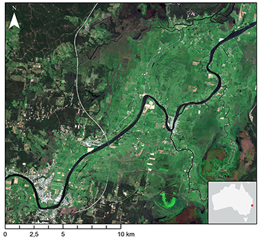
Figure 1. The study area in the vicinity of the city Kempsey, near the outlet of Macleay River on the Mid North Coast in New South Wales, Australia. Background: True-colour combination of bands, R-band 4, G-band 3, B-band 2 from Sentinel-2 MSI imagery from January 25, 2021

I. Materials and methods

11To address the research questions, we implemented a multiple-step procedure of image pre-processing and analysis (Figure 2), starting with image classification for land cover mapping and follow-up by near-real-time flood extent mapping.

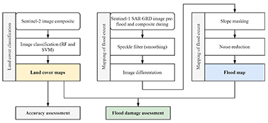
Figure 2. Flowchart illustrating data processing and end results

A. Sentinel data

12In this study, we relied on the European Space Agency’s Copernicus Sentinel-1 and Sentinel-2 data (Table 1). Sentinel-1 satellite provides imagery from a dual-polarisation C-band Synthetic Aperture Radar (C-SAR) instrument. It allows to obtain all-weather and day-and-night imagery in high resolution and has a temporal resolution of nine days. The Sentinel-1 C-SAR constellation provides images with high reliability with improved geographical coverage, short revisit time, observations through the clouds and rapid distribution of data. This all makes Sentinel-1 C-SAR very well suited for emergency mapping (ESA, 2021b)

13Signal processing with the C-SAR instrument uses the magnitude and phase of received signals through several consecutive pulses from elements on the Earth’s surface to create an image (ESA, 2021a). With changes in the line-of-sight direction along the radar trajectory, the effect of lengthening the antenna is produced through signal processing, thus creating a synthetic aperture. Using C-SAR, the achievable azimuth resolution equals one-half the length of the real antenna. This is not dependent on the altitude (ESA, 2021a).

14Each Sentinel-1 C-SAR image has four different polarisation bands:

15• Horizontal Transmit – Horizontal Receive Polarisation (HH), a mode of radar polarisation where the electro-field microwaves are oriented in the horizontal plane in both the signal transmission and the reception of the radar antenna;

16• Vertical Transmit – Vertical Receive Polarisation (VV), a mode of radar polarisation where the electro-field microwaves are oriented in the vertical plane for both the signal transmission and the reception of the radar antenna;

17• Horizontal Transmit – Vertical Receive Polarisation (HV), a radar polarisation mode, where the electro-field microwaves are oriented in the horizontal plane, while the vertically polarised electric field of the backscattered energy is received by the radar antenna;

18• Vertical Transmit – Horizontal Receive Polarisation (VH), a radar polarisation mode, where the electro-field microwaves are oriented in the vertical plane, while the horizontal polarised electric field of the backscattered energy is received by the radar antenna (ESA, 2021a).

Platform	Instrument	Image dates
Sentinel-1	C-SAR	07-03-2021 / 18-03-2021 / 24-03-2021
Sentinel-2	MSI Level-2A	01-12-2020 – 28-02-2021

Table 1. Data sets used in the study

19The optical Sentinel-2 satellite carries a wide-swath optical instrument that delivers high resolution imagery through multispectral imaging and has a temporal resolution of 10 days. The Sentinel-2 Multispectral Instrument (MSI) is delivering high radiometric resolution, which increases the capacity to detect and differentiate light intensity and differences in surface reflectance (ESA, 2021c; ESA, 2021d). This information is represented through 13 different spectral bands; four bands at 10 meters spatial resolution, six bands at 20 meters spatial resolution and three bands at 60 meters spatial resolution. With its high spatial and radiometric resolution, Sentinel-2 MSI data are ideal for monitoring different types of ground cover such as soil, vegetation, water and ice (ESA, 2021c; ESA, 2021d). 

B. Land cover mapping with Sentinel-2 MSI Level-2A data

1. Reference composite for land cover mapping

20To estimate flood damage, a land cover map was produced with Sentinel-2 MSI Level-2A data and machine learning techniques in GEE. Firstly, we created a summer image composite from January 12, 2020, to February 28, 2021, hence representing the land conditions prior to the flood event. The image composite consisted of images with a cloud coverage below 2 % and represented median values of the blue (490 nm), green (560 nm), red (665 nm) and near-infrared (842 nm) in the collection. This image composite was later classified.

2. Training data

21The production of training data was performed with a random sampling of points in QGIS software (QGIS, 2021) within the study area. The thematic classes were assigned to the sampled points by visual interpretation of Sentinel-2 MSI Level-2A imagery available via the GEE Data Catalog (Table 2). The training sample size should theoretically represent approximately 0.25 % of the total study area, as the size of the sample can influence the performance of the RF classifier (Belgiu & Drăguţ, 2016). In this case, 0.25 % of the study area corresponds approximately to 12 200 pixels. Due to temporal constraints, a sample size of 550 points was used for training, where 500 points were generated randomly and approximately 50 were generated through a stratified random sampling in the rarer areas to have at least 50 points for each class.

	Training points	Validation points	Class description	Land cover on Sentinel-2 satellite imagery (visible, true colour combination of bands, R-band 4, G-band 3, B-band 2)
Forest	109	84	Trees, shrub
Grassland	282	182	Grass, wetland, bare soil
Cropland	50	55	Farmland
Urban	52	59	Roads, bridges, buildings
Water	51	58	Rivers, lakes, ponds
Total	544	438

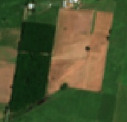
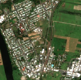
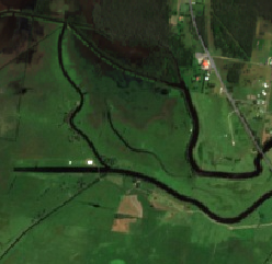
Table 2. Land cover classification catalogue

3. Validation data

22Often agricultural landscapes are not random and possess a degree of spatial autocorrelation. Therefore, it is important to reduce a bias introduced by spatial autocorrelation to increase the reliability of the validation. The correlation coefficient Moran’s I, measures the overall spatial correlation in a given dataset, resulting in a value that ranges from 1 (indicating a strong positive spatial autocorrelation) and – 1 (indicating a strong negative spatial autocorrelation). A value near 0 is desirable as it indicates perfect randomness and thus no bias (Esri, 2021).

23The set of reference data used for cross-validation of the classification methods was created by sampling points from high resolution Sentinel-2 imagery. First, to determine the minimum distance between reference points required to reduce bias, Moran’s I was used. A Moran’s I-value near 0 occurred close to a pixel distance of 100, and as such, this is technically what should have been used when randomly generating reference points. Because of the size of the study area, it was not possible to use this length, as too few points would be generated with the desired sample size. Instead, a distance of 10 pixels was used, as this let us generate the desired number of samples, which reduced spatial autocorrelation by 50 % from 0.8 to 0.4.

24Olofsson et al. (2014) recommended a minimum sample size of 50 to 100 per class. In this study, 300 points were randomly generated, and classes were assigned using high resolution imagery from Google Earth and Sentinel-2. Underrepresented classes, such as cropland, urban and water, were brought up to a minimum of 50 via stratified random sampling leaving the distribution shown in Table 2.

254. Applying machine learning classifiers

26To produce land cover classifications, two classifiers, RF and SVM, were tested with different parameters. RF is a classification method that produces multiple decision trees using a random subset of training data and variables (Belgiu & Drăguţ, 2016). This approach is known as bagging, i.e. where a fraction of the training data is randomly selected to train each decision tree. Together with the number of tree parameters, bagging contributes to reducing the complexity of the models that overfit the training data. Overall, the RF classification method provides a good approximation of the results and furthermore gives estimates about the importance of each used classification variable (Belgiu & Drăguţ, 2016). SVM is a non-parametric classifier that uses support vectors based on training data to separate classes that are hard to distinguish by fitting the data to a hyperplane in n-dimensions (Prishchepov et al., 2012). For SVM to be reliable, it requires error-free training data, as errors will be significantly reflected in the end results (Foody, 2015). If SVM is not tuned correctly, SVM tends to overfit data during the training process, thus making training data fit very well, while having difficulties with correct model approximation (Foody & Mathur, 2004).

27When working with RF, there are several parameters that can be set to configure RF. Among them: the number of trees to be generated (Ntree) and the number of variables to be selected and tested for the best node-split when growing trees (Mtry). Between the two, the previous study showed that classification accuracy was less sensitive to Ntree than Mtry (Belgiu & Drăguţ, 2016). Theoretically, Ntree can be as large as possible since the classification method is computationally efficient and does not tend to over fit. A value of 500 is commonly used, although this number should be taken with caution depending on the complexity of classified data (Belgiu & Drăguţ, 2016). However, often out-of-bag accuracy may indicate that fewer trees are required to classify satellite imagery. Mtry is usually calculated by taking the square root of the number of input variables, although it can be set to all variables at a cost to computation time (Belgiu & Drăguţ, 2016). In our case, acceptable results with the RF model were reached once the Ntree parameter was set to 50, while the Mtry parameter was set to 2.

28When applying SVM as a classifier, the main adjustable parameters are gamma and cost (C), which can be tuned in order to boost image classification accuracy. The gamma parameter defines the length of the radius of the influence of a single training sample. A low gamma value means that the influence is far reaching, while on the contrary, a high gamma value equals the range of influence to be shorter. The SVM model is very sensitive to the gamma parameter (Huang et al., 2002). If the gamma value is too low, the complexity of the training data will not be captured as the influence of a single training sample would influence the entire training data set (Foody & Mathur, 2004). On the contrary, if the gamma value is too high, the area of influence would be constrained to the training sample itself. The parameter C acts as a regulator within the SVM classifier that influences training accuracy and computational time. If the C parameter is set to a high value, the amount of support vectors is lowered. This will result in faster computation time while decreasing the training accuracy. Contrarily, a low C value increases the number of support vectors, thus enhancing training accuracy on the cost of longer computational time (scikit-learn, 2021). For this study, the best SVM model had the gamma parameter set to 700 and the applied C parameter set to 10.

29While working with both classifiers, many different qualified values were tested for each optimised parameter, which resulted in models with a steadily increasing accuracy until no further optimisation could be seen. The three RF main parameters, namely, the number of trees, bagging size and number of variables, were tuned. For SVM in GEE, changing kernel Type to Radial Basis Function (RBF) allowed for further fine-tuning of the gamma and cost parameters. Running the classifiers in GEE allowed for an efficient performance evaluation of the classifiers with different parameter settings as the computational cost for each classification took only a few seconds. Evaluating the classifications based on overall accuracy from our validation data made it possible to quickly identify the best performing classifications.

C. Accuracy assessment of RF and SVM mappings

30To assess classification accuracy using validation points, we calculated:

31• overall accuracy (OA), which tells us, out of all the reference data used, what proportion was mapped correctly by the model;

32• producer’s accuracy (PA), which describes how often reference features in a class are actually shown on the classified map;

33• user’s accuracy (UA), which conveys how often a class on the classified map will be present in the reference data (Congalton, 1991).

34Producer’s accuracy is often called estimation of the degree of omission (errors of omission – EOO), when validating data that was missed from a correct class of the classified map. User’s accuracy is often called a degree of errors of commission (EOC), when a fraction of validation data is predicted to be in a class in which they do not belong (Congalton & Green, 2020; Olofsson et al., 2014). The calculated error matrix between classification and validation data allows the estimation of OA, PA and UA and also provides the basis for estimating error-adjusted area estimates (Olofsson et al., 2014).

1. Error-adjusted area estimates

35To reduce some of the differences between the “true” area approximated by a validation sample and the areas obtained from the classified maps, which contain misclassification errors, area proportion adjustment was implemented based on the confusion matrix of the best RF and SVM performance after cross-validation. Firstly, an error matrix with estimated area proportions was calculated, based on the distribution of mapped pixels for each class. Then, for error-adjusted areas, the standard errors at a 95 % confidence interval were calculated per class, giving a standard error estimate in pixels. Lastly, user’s and producer’s accuracies were calculated for each thematic based on the area-adjusted proportions and a new OA is calculated for both mappings.

2. McNemar test

36The non-parametric McNemar test was used for pairwise comparison of classification outcomes with RF and SVM classifiers. This was done to evaluate whether one classification was significantly better (i.e. more accurate) than the other (Prishchepov et al., 2012). The null hypothesis (i.e. the accuracies of classified maps with RF and SVM are equal) was tested at a 95 % confidence interval. The Chi-squared test was performed based upon a 2 x 2 contingency table where correct and incorrect class allocations for each classifier were being reported in pairs (Foody, 2004; Kavzoglu, 2017). The test was conducted through the following equation:

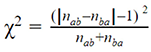
37where nab is the number of pixels misclassified by method a, but classified correctly by method b, and nba is the number of pixels misclassified by method b, but classified correctly by method a (Kavzoglu, 2017). 

D. Quantifying and mapping flood extent with Sentinel-1 SAR GRD data

38The flood mapping analysis was performed in Google Earth Engine (GEE), where three images from the image collection Sentinel-1 SAR GRD (Ground Range Detected) were used (Table 1): one image from March 7, before the flood event, and two images from March 18 and 24, during the event. In both cases, vertical-horizontal (VH) dual polarisation was used with a selected spatial resolution of 10 meters. First, the two images from during the event were concatenated into a minimum value composite to capture the full extent of the floods. Then, a smoothing filter, using the function focal mean and a smoothing radius of 100 meters, was applied both to the before-flood image and the during-flood composite to reduce radar speckle. Second, the image difference was performed between the before-flood and during-flood images to capture change. A predefined difference threshold was applied to create a binary difference image and mask the flood extent. The threshold was set based on local water reflectance values. Also, flood-pixels connected to fewer than eight other pixels were masked out to reduce noise and areas with a slope of > 5 % by importing a digital elevation model (DEM) dataset from WWF – HydroSHEDS (Lehner et al., 2008) into GEE to produce the final flood extent mask. The resulting flood extent map was then later used for assessing flood damages when combined with land cover classifications.

39As a final step, our flood extent mask from Sentinel-1 SAR was overlaid with our best RF and SVM classifications, which allowed us to create a damage assessment of the total area in hectares affected by flood per class. This final product can be used to further assess damages made, for instance, to urban and agricultural areas.

II. Results

A. Land cover classification: optimal parameters and associated land cover maps

40Several important parameters were tested to tune the RF and SVM classifiers. The best classification was chosen by looking at the overall accuracy using validation data. For RF, the highest overall accuracy was reached with the following parameter settings: Ntree = 50; Ntry = 2; bagging fraction = 0.5. A slight improvement in the overall accuracy up from 84.7 % to 85.2 % was reached with these settings. For SVM, the overall accuracy increased substantially from 64.4 % to 88.1 % using gamma = 700 and cost = 10 (Table 6) instead of the default settings of gamma = 1 and cost = 1, thus outperforming the best RF classification.

41Figure 3 illustrates the best RF and SVM classifications for the study area. In both cases, the land cover was dominated by the grassland and forest classes, with clusters of urban areas as well as occurrences of cropland along the river. In terms of distribution, the only expressive difference between the classifications was in the urban class, which constituted 5.5 % of the total area in the RF-based map while only covering 4.5 % of the SVM-based map. The OAs were 85.2 % for RF and 88.1 % for SVM, respectively. One noticeable difference between the two classifications was the urban class affected by floods. RF identified 4.74 hectares for urban thematic class (UA = 82.8 %), while SVM identified 3.61 hectares (UA = 86.9 %). Pairwise comparison of the RF and SVM classifiers, with McNemar test at a 95 % confidence interval, resulted in a p-value of 0.052, which was very close to the point where the null hypothesis can be rejected ( = 0.05). Based on the decision to follow the p-value cut-off of 0.05, the two classified maps were statistically similar (Figure 3).

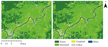
Figure 3. Best RF (A) and SVM (B) land cover classifications (image composite Dec. 2020 - Feb. 2021)

B. Accuracy assessment

1. Random Forest (RF)

42For RF (Table 3), PA and UA accuracies above 80 % were reached in all classes except the cropland thematic class, with PA of 65.5 % and UA of 70.6 %. At the same time, the urban thematic class was classified with PA of 89.8 % and UA of 82.2 %. Implementing error adjustments of calculated areas to errors induced in the product classification did not affect the overall accuracy, however it changed PA for all classes, and most noticeably for the cropland thematic class when PA decreased to just 39.5 % (Table 4).

Validation data
		Forest	Grassland	Cropland	Urban	Water	TOT	UA (%)
Classification data	Forest	69	9	0	0	0	78	88.5
	Grassland	15	162	12	1	2	192	84.4
	Cropland	0	7	36	5	3	51	70.6
	Urban	0	4	7	53	0	64	82.8
	Water	0	0	0	0	53	53	100.0
	TOT	84	182	55	59	58	438
	PA (%)	82.1	89.0	65.5	89.8	91.4		85.2

Table 3. Confusion matrix between best RF classification and validation data

	Forest	Grassland	Cropland	Urban	Water
PA (%)	82.0	93.3	39.5	86.1	73.3
UA (%)	88.5	84.4	70.6	82.8	100.0
OA (%)	85.2

Table 4. Producer’s and user’s accuracies of the best RF classification after error adjustment of area estimates

2. Support Vector Machines (SVM)

43SVM resulted in PA and UA classification accuracies for most of the thematic classes above 75 % (Table 5). For instance, for the cropland class PA was 78.2 % and UA was 79.6 %. For the urban class, PA for RF and SVM classifications were similar, but UA for the urban class was higher with SVM classifier (86.9 %). After error adjustment, PA for the cropland classes decreased to 51.9 %. Also, PU for the urban class decreased from 86.9 % to 80.5 %. At the same time, PA and UA accuracies for the grassland class increased (Table 6).

	Validation data
		Forest	Grassland	Cropland	Urban	Water	TOT	UA (%)
Classification data	Forest	72	6	0	0	0	80	90.0
	Grassland	12	165	8	2	2	190	86.8
	Cropland	0	7	43	4	3	54	79.6
	Urban	0	4	4	53	0	61	86.9
	Water	0	0	0	0	53	53	100.0
	TOT	84	182	55	59	58	438
	PA (%)	85.7	90.7	78.2	89.8	91.4		88.1

Table 5. Confusion matrix between best SVM classification and validation data

	Forest	Grassland	Cropland	Urban	Water
PA (%)	85.1	95.3	51.9	80.5	74.2
UA (%)	92.3	87.3	75.4	86.9	100.0
OA (%)	88.4

Table 6. Producer’s and user’s accuracies of the best RF classification after error adjustment of area estimates

3. Flood mapping and damage assessment

44The flood map based on Sentinel-1 SAR data showed extensive flood throughout the study area (Figure 4). In total, 17 988 hectares of land were flooded between March 18 and 24, 2021 (Table 7), of which a large majority of flooded areas corresponded to grasslands – approximately 90 % of the total flooded area (Table 7). Conversely, the least affected class was urban – approximately 4 – 5 % of the total flooded area, with the cities of Kempsey and Frederickton. At the same time, approximately 16 – 18 % of the total urban area was affected by flood (Table 7), while approximately 33 – 42 % of the total cropland area was affected. The study area was primarily composed of grasslands, of which approximately 51 % were affected by flood. The forest thematic class was the least affected by flood; approximately 7 % of its total area was affected by floods.

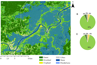
Figure 4. Flooded area (18 - 24 March 2021) overlaid over the best SVM-classified map (A). Percentage of land cover affected by floods estimated from RF-classified map (B) and SVM-classified maps (C)

	Forest	Grassland	Cropland	Urban	Water	Total
Best RF	945 (7.7 %)	15,596 (51 %)	863 (42.3 %)	474 (17.7 %)	110	17,988
Best SVM	802 (6.6 %)	15,990 (51.5 %)	701 (33.6 %)	361 (16.1 %)	133	17,988

Table 7. Land cover types affected by flood in hectares (percentage of flooded area within each class in brackets)

Conclusions

A. Discussion

45Through this study, we successfully mapped both land cover types and flooded areas during the March 2021 event in New South Wales (Australia). This allowed us to synergistically assess the areas affected by flood in the study area, revealing where the flood had the largest impact. When estimating the flood damage done to the area, it bears most relevant to consider the scale of flooded urban and cropland areas as these land uses have the highest economic value and affect larger parts of the population directly (Lambin, 2012; Kok et al., 2014). Even though grassland was primarily affected by flood, there were also alarmingly large cropland and urban areas that were affected in March 2021, which resulted in local economic and personal losses (Kurmelovs, 2021). Continuing to map emergencies such as these and taking preventive measures to safeguard vulnerable areas, therefore, bears great importance for limiting or preventing future impoverishment.

46When performing emergency mapping, data availability and quality are of utmost importance. In the case of near real-time mapping of floods, dense cloud covers are, due to the inherent nature of the disaster, frequently co-occurring with it. These circumstances made it infeasible to use optical data. Therefore, radar data from the Sentinel-1 C-SAR were used specifically because of its ability to penetrate clouds, limiting the production of flood mapping to only one type of data. It is worth noticing that Sentinel-1 C-SAR data are available at a nine-day interval which could be argued as being a data availability flaw in the context of ongoing emergency mapping, the temporal frequency of which could be improved in the future.

47Copernicus EMS-RM uses both optical and radar satellite imagery from the Sentinel missions or other contributing providers. For rapid mapping imagery acquisitions, ESA has a mechanism called REACT, which works as a 24/7 fast-track mode for data retrieval in emergency situations (Ajmar et al., 2017). In this case, optical imagery covering the dates of the event at a high resolution could not be gathered; the applied Sentinel-1 C-SAR data was not compared with any alternatives. Comparing our flood mapping extent product with one of Copernicus EMS-RM’s post-event maps, the Copernicus grading map (Copernicus, 2021), the results seem to align quite well. The Copernicus grading map consists of a high resolution optical satellite image as background as well as topographical features, a detailed description of the event and a damage assessment.

48In recent years the use of RF and SVM for land cover classification has increased significantly, as these classifiers produce high accuracies (Thanh Noi & Kappas, 2017; Sheykhmousa et al., 2020). Our land cover classifications had an overall accuracy of 85.2 % using the RF classifier and 88.1 % using the SVM classifier. We achieved plausible classification accuracies. For instance, the urban thematic land cover class reached a user’s accuracy of 82.8 % with RF, and 86.9 % with SVM, while PA was 89.8 % for both classified maps. Other studies also applied Sentinel-2 imagery for land cover classification with good classification results (Huang & Jin, 2020; Chaves et al., 2020). Generally one considerable challenge is to attain a high accuracy for multimodal classes such as the cropland and urban thematic classes (Valero et al., 2016; Hu et al., 2021).

49Training and validation data were collected by looking at both natural and false colour composites of Sentinel-2 imagery, where it can be challenging to identify the land cover with a resolution of 10 meters. The grassland and cropland thematic classes were especially difficult to distinguish from each other as, spectrally, they can look very similar when comparing both harvested cropland and dry grass, or comparing growing crops versus healthy grasses. These difficulties are also seen in our results on accuracy assessment. Generally, cropland accuracies were lower, which is probably due to a combination of errors in training and validation data and spectral similarities leading to errors made by the classifiers. From a damage assessment point of view, we were particularly pleased to obtain the urban land cover thematic class with high classification accuracy. The cropland thematic class also performed statistically significantly more accurately with SVM than RF. However, after making error adjustments of area estimates, the cropland accuracies decreased for both SVM and RF classification. Still, an error-adjusted overall accuracy of 8.4 % with SVM would probably be good enough to use for damage assessments in emergency mapping. Considering the scale of flooded areas, our focus was on the cropland and urban thematic classes as these represent the most valuable land cover types upon which flood would impose the most economic damage. Natural flood events cannot be prevented, but timely remote sensing tools and machine learning techniques, combined with cloud-computing platforms, such as Google Earth Engine, can be useful for estimating flood damages in emergency mapping as well as disaster management when applied and tuned correctly.

B. Limitations and outlook

50When it comes to land cover classifications of remotely-sensed images, several limitations may impose classification uncertainties. Having in situ observations at hand is always beneficial in terms of classification accuracy. Any research, however, will have limitations regarding funds and time, which creates gaps in knowledge about the actual conditions in the study area. In areas with diverse land cover types, one of the critical choices to be made relates to the level of details to be contained in the final map, which should be driven by the message or information that the map is meant to convey. Since the objective of this analysis was to detect flood over managed area, wetlands were included in the grasslands class, as both types of land cover were assumed to be unmanaged and because the spectral signature was similar in many cases. However, part of the grassland areas is in fact managed grasslands for grazing cattle, which presents an additional source of local economic losses. Therefore further refinement of our mapping results should include a distinction between managed and unmanaged grasslands.

51Throughout the remote sensing literature, the R statistical software (R Core Team, 2021) is a commonly used open-source environment for classification with RF and SVM (Sheykhmousa et al., 2020). However, GEE was, here, chosen as the primary platform for data pre-processing and analysis. Compared to environments such as R and Python, GEE cloud environment made the pre-processing of Sentinel-1 and Sentinel-2 data faster, as pre-processing steps such as e.g. calibration and corrections were already made in the SAR GRD dataset. The availability of auxiliary data in GEE also facilitated other pre-processing steps, e.g. masking out elevated and rugged terrain for flood extent mapping. Finally, a comprehensive step-by-step GEE flood mapping and Damage Assessment procedure (UNOOSA, 2021) was an important source of information when producing our own flood mapping workflow. By combining the flood extent workflow and the land cover classification workflow into a single script in GEE, the final damage assessment product can be created in one single run. However, several limitations to GEE should be reported. Function availability and documentation are currently not as comprehensive as in other programs e.g. R statistical software. The RF feature importance parameter is an example of a currently missing function in GEE. Yet, GEE has a continuously growing community of engaged users and it continues to evolve with new functions and applications becoming available every week.

52The method employed in this study is universal and could therefore be transferred to other parts of the globe in which flood disasters pose a threat. It would be especially relevant in areas that are projected to receive more floods due to climate change, such as Southeast Asia, East Asia, South America, Central Africa and parts of Western Europe (Hirabayashi et al., 2013).

Notes and acknowledgement

53This work reflects different elements of active learning and problem-oriented teaching as a part of the 2020 - 2021 master course Remote Sensing in Land Science Studies NIGK17012U (https://kurser.ku.dk/course/nigk17012u). It illustrates the students’ ability to address a selected topic of their choice (here emergency flood mapping) by implementing acquired knowledge during the class on (1) advanced image classification with machine learning techniques; (2) state-of-the-art accuracy assessment; (3) cloud computation; (4) multisource satellite image fusion. Rasmus P. Meyer, Mathias P. Schødt and Mikkel G. Søgaard designed the research, conducted the analyses and were actively engaged in writing. Alexander V. Prishchepov and Stéphanie Horion instructed during the class, supervised the research and contributed to writing. The Google Earth Engine script for emergency mapping of floods developed here is available at: https://code.earthengine.google.com/6e425efa3ac61c5b0a7bcfd6cc05cce7.

References

54ABARES (2021). About my region – Mid North Coast New South Wales. Australian Bureau of Agricultural and Resource Economics and Sciences. Australian Government. https://www.agriculture.gov.au/abares/research-topics/aboutmyregion/mid-north-coast. Retrieved April 7, 2021.

55Ajmar, A., Boccardo, P., Broglia, M., Kucera, J., Giulio-Tonolo, F. & Wania, A. (2017). Response to Flood Events: The Role of Satellite-based Emergency Mapping and the Experience of the Copernicus Emergency Management Service. In Molinari, D., Menoni, S. & Ballio, F. (eds.), Geophysical Monograph Series. Hoboken: John Wiley & Sons, Inc., 211 – 228 https://doi.org/10.1002/9781119217930.ch14

56Amitrano, D., Di Martino, G., Iodice, A., Riccio, D. & Ruello, G. (2018). Unsupervised Rapid Flood Mapping Using Sentinel-1 GRD SAR Images. IEEE Transactions on Geoscience and Remote Sensing, 56 (6), 3290 – 3299. https://doi.org/10.1109/TGRS.2018.2797536

57Belgiu, M. & Drăguţ, L. (2016). Random forest in remote sensing: A review of applications and future directions. ISPRS Journal of Photogrammetry and Remote Sensing, 114, 24 – 31. https://doi.org/10.1016/j.isprsjprs.2016.01.011

58Boccardo, P. & Giulio Tonolo, F. (2015). Remote Sensing Role in Emergency Mapping for Disaster Response. In Lollino, G., Manconi, A., Guzzetti, F., Culshaw, M., Bobrowsky, P. & Luino, F. (eds.), Engineering Geology for Society and Territory – Volume 5. New York : Springer International Publishing, 17 – 24. https://doi.org/10.1007/978-3-319-09048-1_3

59BOM (2021). Climate Data Online. Bureau of Meteorology. Australian Government. http://www.bom.gov.au/climate/data/index.shtml. Retrieved April 7, 2021.

60Brivio, P.A., Colombo, R., Maggi, M. & Tomasoni, R. (2002). Integration of remote sensing data and GIS for accurate mapping of flooded areas. International Journal of Remote Sensing, 23 (3), 429 – 441. https://doi.org/10.1080/01431160010014729

61Chaves, M.E.D., Picoli, M.C.A. & Sanches, I.D. (2020). Recent Applications of Landsat 8/OLI and Sentinel-2/MSI for Land Use and Land Cover Mapping: A Systematic Review. Remote Sensing, 12 (18). https://doi.org/10.3390/rs12183062

62Congalton, R.G. (1991). A review of assessing the accuracy of classifications of remotely sensed data. Remote Sensing of Environment, 37 (1), 35 – 46. https://doi.org/10.1016/0034-4257(91)90048-B

63Congalton, R.G. & Green, K. (2020). Assessing the Accuracy of Remotely Sensed Data: Principles and Practices. Third Edition. London: Taylor & Francis Group.

64Copernicus (2021). [EMSR504] Kempsey: Grading Product, version 2, release 1, RTP Map #01. European Commission. https://emergency.copernicus.eu/mapping/ems-product-component/EMSR504_AOI01_GRA_PRODUCT_r1_RTP01/2. Retrieved April 4, 2021.

65Esri. (2021). How Spatial Autocorrelation (Global Moran’s I) works—ArcGIS Pro | Documentation. Esri. https://pro.arcgis.com/en/pro-app/latest/tool-reference/spatial-statistics/h-how-spatial-autocorrelation-moran-s-i-spatial-st.htm. Retrieved April 5, 2021.

66ESA (2021a). User Guides—Sentinel-1 SAR - Definitions—Sentinel Online. European Space Agency. https://sentinel.esa.int/web/sentinel/user-guides/sentinel-1-sar/definitions. Retrieved April 5, 2021.

67ESA (2021b). User Guides—Sentinel-1 SAR - Overview—Sentinel Online. European Space Agency. https://sentinel.esa.int/web/sentinel/user-guides/sentinel-1-sar/overview. Retrieved April 5, 2021.

68ESA (2021c). User Guides—Sentinel-2 MSI - Overview—Sentinel Online. European Space Agency. https://sentinel.esa.int/web/sentinel/user-guides/sentinel-2-msi/overview. Retrieved April 5, 2021.

69ESA (2021d). User Guides—Sentinel-2 MSI - Radiometric—Resolutions—Sentinel Online. European Space Agency. https://sentinel.esa.int/web/sentinel/user-guides/sentinel-2-msi/resolutions/radiometric. Retrieved April 5, 2021.

70Feng, Q., Liu, J. & Gong, J. (2015). Urban Flood Mapping Based on Unmanned Aerial Vehicle Remote Sensing and Random Forest Classifier—A Case of Yuyao, China. Water, 7 (12), 1437 – 1455. https://doi.org/10.3390/w7041437

71Foody, G.M. (2004). Thematic Map Comparison. Photogrammetric Engineering & Remote Sensing, 70 (5), 627 – 633. https://doi.org/10.14358/PERS.70.5.627

72Foody, G.M. (2015). The effect of mis-labeled training data on the accuracy of supervised image classification by SVM. 2015 IEEE International Geoscience and Remote Sensing Symposium (IGARSS). 4987 – 4990. https://doi.org/10.1109/IGARSS.2015.7326952

73Foody, G.M. & Mathur, A. (2004). A relative evaluation of multiclass image classification by support vector machines. IEEE Transactions on Geoscience and Remote Sensing, 42 (6), 1335 – 1343. https://doi.org/10.1109/TGRS.2004.827257

74Gergis, J. (2021). Yes, Australia is a land of flooding rains. But climate change could be making it worse. The Conversation. http://theconversation.com/yes-australia-is-a-land-of-flooding-rains-but-climate-change-could-be-making-it-worse-157586. Retrieved October 3, 2021.

75Gibson, R., Danaher, T., Hehir, W. & Collins, L. (2020). A remote sensing approach to mapping fire severity in south-eastern Australia using sentinel 2 and random forest. Remote Sensing of Environment, 240, 111702. https://doi.org/10.1016/j.rse.2020.111702

76Hirabayashi, Y., Mahendran, R., Koirala, S., Konoshima, L., Yamazaki, D., Watanabe, S., Kim, H. & Kanae, S. (2013). Global flood risk under climate change. Nature Climate Change, 3 (9), 816 – 821. https://doi.org/10.1038/nclimate1911

77Hu, B., Xu, Y., Huang, X., Cheng, Q., Ding, Q., Bai, L. & Li, Y. (2021). Improving Urban Land Cover Classification with Combined Use of Sentinel-2 and Sentinel-1 Imagery. ISPRS International Journal of Geo-Information, 10 (8). https://doi.org/10.3390/ijgi10080533

78Huang, C., Davis, L.S.,- & Townshend, J.R.G. (2002). An assessment of support vector machines for land cover classification. International Journal of Remote Sensing, 23 (4), 725 – 749. https://doi.org/10.1080/01431160110040323

79Huang, M. & Jin, S. (2020). Rapid Flood Mapping and Evaluation with a Supervised Classifier and Change Detection in Shouguang Using Sentinel-1 SAR and Sentinel-2 Optical Data. Remote Sensing, 12 (13). https://doi.org/10.3390/rs12132073

80IPCC (2021). Climate Change 2021: The Physical Science Basis. In Masson-Delmotte, V., Zhai, P., Pirani, A., Connors, S.L., Péan, C., Berger, S., Caud, N., Chen, Y., Goldfarb, L., Gomis, M.I., Huang, M., Leitzell, K., Lonnoy, E., Matthews, J.B.R., Maycock, T.K., Waterfield, T., Yelekçi, O., Yu, R. & Zhou, B. (eds.), Contribution of Working Group I to the Sixth Assessment Report of the Intergovernmental Panel on Climate Change. Cambridge: University Press.

81Kavzoglu, T. (2017). Object-Oriented Random Forest for High Resolution Land Cover Mapping Using Quickbird-2 Imagery. In Samui, P., Roy, S.S. & Balas, V.E. (eds.), Handbook of Neural Computation. Washington D.C.: Academic Press, 607-619. https://doi.org/10.1016/B978-0-12-811318-9.00033-8

82Khatami, R., Mountrakis, G. & Stehman, S.V. (2016). A meta-analysis of remote sensing research on supervised pixel-based land-cover image classification processes: General guidelines for practitioners and future research. Remote Sensing of Environment, 177, 89 – 100. https://doi.org/10.1016/j.rse.2016.02.028

83Kok, N., Monkkonen, P. & Quigley, J.M. (2014). Land use regulations and the value of land and housing: An intra-metropolitan analysis. Journal of Urban Economics, 81, 136 – 148. https://doi.org/10.1016/j.jue.2014.03.004

84Kurmelovs, R. (2021). Fire and flood: “Whole areas of Australia will be uninsurable.” The Guardian, April 1, 2021. https://www.theguardian.com/australia-news/2021/apr/02/fire-and-flood-whole-areas-of-australia-will-be-uninsurable

85Lambin, E.F. (2012). Global land availability: Malthus versus Ricardo. Global Food Security, 1 (2), 83 – 87. https://doi.org/10.1016/j.gfs.2012.11.002

86Lehner, B., Verdin, K. & Jarvis, A. (2008). New Global Hydrography Derived From Spaceborne Elevation Data. Eos, Transactions American Geophysical Union, 89 (10), 93. https://doi.org/10.1029/2008EO100001

87McCabe, M.F., Rodell, M., Alsdorf, D.E., Miralles, D.G., Uijlenhoet, R., Wagner, W., Lucieer, A., Houborg, R., Verhoest, N.E.C., Franz, T.E., Shi, J., Gao, H. & Wood, E.F. (2017). The future of Earth observation in hydrology. Hydrology and Earth System Sciences, 21 (7), 3879 – 3914. https://doi.org/10.5194/hess-21-3879-2017

88NASA Earth Observatory (2021). Historic Floods in New South Wales. NASA. https://earthobservatory.nasa.gov/images/148093/historic-floods-in-new-south-wales. Retrieved March 3, 2021.

89Notti, D., Giordan, D., Caló, F., Pepe, A., Zucca, F. & Galve, J. (2018). Potential and Limitations of Open Satellite Data for Flood Mapping. Remote Sensing, 10 (11), 1673. https://doi.org/10.3390/rs10111673

90Olofsson, P., Foody, G.M., Herold, M., Stehman, S.V., Woodcock, C.E. & Wulder, M.A. (2014). Good practices for estimating area and assessing accuracy of land change. Remote Sensing of Environment, 148, 42 – 57. https://doi.org/10.1016/j.rse.2014.02.015

91Prishchepov, A.V., Radeloff, V.C., Dubinin, M. & Alcantara, C. (2012). The effect of Landsat ETM/ETM + image acquisition dates on the detection of agricultural land abandonment in Eastern Europe. Remote Sensing of Environment, 126, 195 – 209. https://doi.org/10.1016/j.rse.2012.08.017

92QGIS (2021). QGIS 3.16. QGIS Geographic Information System. QGIS Association. http://www.qgis.org. Retrieved October 23, 2021.

93R Core Team (2021). R: A language and environment for statistical computing. Vienna: R Foundation for Statistical Computing. https://www.R-project.org/. Retrieved October 23, 2021.

94scikit-learn. (2021). RBF SVM parameters. scikit-learn. https://scikit-learn.org/stable/auto_examples/svm/plot_rbf_parameters.html. Retrieved April 4, 2021.

95Sheykhmousa, M., Mahdianpari, M., Ghanbari, H., Mohammadimanesh, F., Ghamisi, P. & Homayouni, S. (2020). Support Vector Machine Versus Random Forest for Remote Sensing Image Classification: A Meta-Analysis and Systematic Review. IEEE Journal of Selected Topics in Applied Earth Observations and Remote Sensing, 13, 6308 – 6325. https://doi.org/10.1109/JSTARS.2020.3026724

96Thanh Noi, P. & Kappas, M. (2017). Comparison of Random Forest, k-Nearest Neighbor, and Support Vector Machine Classifiers for Land Cover Classification Using Sentinel-2 Imagery. Sensors, 18 (2), 18. https://doi.org/10.3390/s18010018

97UNOOSA (2021). Step-by-Step: Recommended Practice: Flood Mapping and Damage Assessment using Sentinel-1 SAR data in Google Earth Engine | UN-SPIDER Knowledge Portal. United Nations Office for Outer Space Affairs. https://un-spider.org/advisory-support/recommended-practices/recommended-practice-google-earth-engine-flood-mapping/step-by-step. Retrieved April 7, 2021.

98Valero, S., Morin, D., Inglada, J., Sepulcre, G., Arias, M., Hagolle, O., Dedieu, G., Bontemps, S., Defourny, P. & Koetz, B. (2016). Production of a Dynamic Cropland Mask by Processing Remote Sensing Image Series at High Temporal and Spatial Resolutions. Remote Sensing, 8 (1), 55. https://doi.org/10.3390/rs8010055.

Om dit artikel te citeren:

Over : Rasmus P. Meyer

Over : Mikkel G. Søgaard

Over : Mathias P. Schødt

Over : Stéphanie Horion

Over : Alexander V. Prishchepov