Guillaume TIMMERMANS, Sébastien DOUTRELOUP, Xavier FETTWEIS & Shady ATTIA

Simulation of long term (1981-2100) evolution of heat waves in Brussels based on mar Regional Model

Résumé

Avec le changement climatique, la Belgique connaît et connaîtra des canicules plus fréquentes et plus sévères, qui sont particulièrement difficile à supporter dans les villes à cause de l’effet d’îlot de chaleur urbain. Dans cette étude, nous nous intéressons à l’évolution des canicules à Bruxelles depuis 1981 ainsi que dans le futur, jusqu’à 2100, à l’aide de simulations climatiques, provenant de modèles globaux affinés par le MAR. Premièrement, une analyse générale de la fiabilité de différents modèles climatiques globaux, et plus particulièrement leur habilité à simuler les canicules à Bruxelles est menée. Ensuite, nous sélectionnons le meilleur modèle et analysons ses projections en termes de futures canicules à Bruxelles, dans le cas du scénario d’émissions de gaz à effet de serre SSP5-8.5. Il apparaît que le modèle sélectionné projette des canicules nettement plus fréquentes, plus longues et plus intenses dans le futur qu’actuellement, dans le cas du SSP5-8.5.

Abstract

With climate change, Belgium is experiencing and will experience more frequent and severe heat waves, which are particularly difficult to withstand in cities due to the urban heat island effect. In this study, we investigate the evolution of heatwaves in Brussels since 1981 and in the future, up to 2100, using climate simulations from global models refined by MAR. Firstly, a general analysis of the reliability of different global climate models, and in particular their ability to simulate heatwaves in Brussels, is conducted. Then, we select the best model and analyze its projections in terms of future heat waves in Brussels, in the case of the SSP5-8.5 greenhouse gas emission scenario. It appears that the selected model projects heatwaves that are significantly more frequent, longer, and more intense in the future than currently, in the case of the SSP5-8.5 scenario.

Table des matières

Introduction

1The effects of heat waves on the health and mortality rates of the urban population in Europe have been a rising concern during the last two decades (Macintre et al., 2018). Heat waves resulting from unusually strong, high-pressure systems are among the costliest climate change-related hazards, causing tens of billions of euros in economic losses globally each year (García-León et al., 2021). Apart from mortality, heat waves have a considerable impact on morbidity (Van Loenhout et al., 2016). Mastrangelo et al. reported an increase in respiratory and heart diseases during heat waves but no increase in circulatory diseases (Mastrangelo et al., 2007). According to the United Nations Intergovernmental Panel on Climate Change IPCC Sixth Assessment Report, failing to characterize heat waves and projections of their future evolution, such losses will worsen in the decades ahead as the planet's temperature continues to rise (IPCC, 2022a).

2The severe impacts of heat waves amply justify the relevance of their study. Indeed, in addition to being, in particular, very detrimental to agriculture and creating favorable conditions for forest fires, heat waves cause excess mortality, as shown, for instance, by Steul et al. (2018) for the 2003 heat wave in Frankfurt. Excess mortality related to the August 2003 heat wave was also observed in France (metropolitan), reaching about 55% between August 1 and August 20, 2003. It should be noted that excess mortality was not spatially uniform since it was about 130% in Paris (in the Île-de-France region), the region most affected (Hémon & Jougla, 2004; Bessemoulin et al., 2004). Laaidi et al. (2012) studied the relationship between mortality and the urban heat island effect during this heat wave in Paris. They found that exposure to high night temperatures on consecutive days increased the likelihood of death during a heat wave. Therefore, it seems that the urban heat island effect, which is mainly felt at night in large cities, plays a key role in excess mortality, hence the interest in studying heat waves in cities. Note that the 2003 heat wave has long been a reference. However, the heat waves of 2019 and 2020 broke records dating back to 2003 (Mievis, 2020; Vautard et al., 2020). We can also mention Pascal et al. (2018), who highlight the influence of high temperature on mortality in French cities.

3In North Western Europe, particularly in Belgium, the heat waves' frequency and intensity are increasing and threatening public health, energy security, and the economy. For example, August 2022 was the warmest month ever recorded in Belgium (IRM, 2022). Indeed, the IPCC (2022b) predicts that Europe, which is already experiencing warming in recent years (Dobrovolný et al., 2010), will have to face more severe heat waves (Vandemeulebroucke et al., 2022). In Belgium, several studies aimed to characterize the weather under climate change conditions and predict future climatic tendencies. Ramon et al. (2020) investigated the different variants of the heating and cooling degree day methods to obtain heating and cooling degree days for building energy use evaluation based on the fifth IPCC assessment report economic scenarios. Doutreloup et al. (2022) developed historical and future weather data for dynamic building simulations in Belgium, focusing on typical and extreme meteorological years and heat waves based on the sixth IPCC assessment report on economic scenarios. However, despite those studies and the availability of weather data provided by the Royal Meteorological Institute of Belgium, there is a scarcity of studies on the future evolution of heat waves concerning thermal comfort in the Belgian context (Attia & Gobin, 2020). The characterization of heat waves and their impact on urban overheating and human life is a pressing priority for local and national governments (Santamouris, 2020). There is a serious need to predict the tendencies of heat waves in the future to develop adaptation and mitigation levels that are integrated and that are heat wave-proof in Northwestern Europe.

4Therefore, this study aims to investigate the evolution of heat waves in the future with a focus on the city of Brussels, which is located on the map in Figure 1. In this context, the study aims to answer the following research questions:

51. How to define heat waves and characterize them based on human thermal comfort requirements, to asses their past evolution and to predict their evolution in the future with rising temperatures?

62. What is and what will the future evolution of heat waves (frequency, duration, severity) be in Brussels, Belgium?

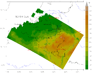
Figure 1. MAR model topography (colour background and dashed black line, both in metres above sea level), localisation of cities (black letters) used in this dataset for Belgium, and localisation of neighbouring countries (in red letters) (Doutreloup et al., 2022).

7The content of this paper is structured as follows: The definitions needed to understand the results and some elements of climate modeling are presented in the methodology section. The results are presented in two parts, the first dealing with the quality of climate models and the second with simulations of a heat wave model in Brussels by 2100. Finally, the conclusion presents a discussion of the results and a reflection on the potential future research.

I. Method

A. Definition and quantification of heat waves

8A heat wave is rather difficult to define universally, as ecosystems and humans do not react in the same way depending on the climate in which they live. In order to make the definition of a heat wave as objective as possible, the definition used here for a "heat wave" was set by Ouzeau et al. (2016) and is based on three temperature thresholds. The thresholds correspond to the quantile of the statistical distribution of daily temperature in a given place, such as a city (more precisely, a weather station). This implies that the definition of a heat wave varies from one city to another. The thresholds are Spic, Sdeb and Sint. Those corresponds to the quantiles 0.995, 0.975 and 0.95, respectively (i.e. the temperatures that are reached or overpassed 0.5%, 2.5% and 5% of the time).

9In addition to varying from one city to another, these thresholds vary as a function of the climate model used (because they do not simulate the same statistical distribution of daily temperature for a given city). The values of the thresholds calculated over the period 1981 - 2010 for Brussels are given in Table 1 as simulated by the regional climate model MAR forced by the ERA5 reanalysis and 3 Earth System Models (ESMs) as explained in Section B.

Threshold - Model	MAR-ERA5	MAR-BCC	MAR-MIR	MAR-MPI
Spic	25.7°C	28.63°C	28.5°C	27.45°C
Sdeb	22.73°C	24.87°C	24.91°C	23.98°C
Sint	21.13°C	22.15°C	23.00°C	22.06°C

Table 1. Temperature thresholds for Brussels city over 1981-2010 as simulated by the MAR model forced by the ERA5 reanalysis and 3 ESMs.

10Based on these thresholds, it is possible to define a heat wave event. If the temperature reaches or overpasses Spic, a ""potential heat wave"" is detected. Then the algorithm considers the beginning of the heat wave as the time when the temperature overpassed Sdeb. It considers that the heat wave ends if the temperature stays below Sdeb for three days or if the temperature passes a rise down Sint. If the duration of the period is superior to or equal to five days, the period is considered a heat wave. An illustration of the definition is available in Figure 2.

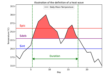
Figure 2. Illustration of the definition of a heat wave and of its intensity.

11When a heat wave event occurs, it can (notably) be characterized by its duration, its mean daily temperature, its maximal daily temperature and its intensity (Ouzeau et al., 2016).

12As expected, the duration is the length of the heat wave in days. The daily mean temperature, in °C, is the sum of each daily mean temperature divided by the length of the heat wave, and the maximal daily temperature, in °C, is the mean daily temperature of the hottest day of the heat wave. Regarding intensity, it is the sum, for each day, of the difference between the daily mean temperature and Sdeb, divided by the difference between Spic and Sdeb. Notice that if a daily mean temperature is below Sdeb, we do not consider this value. The formula is given in Equation 1 (Ouzeau et al., 2016).

13Where Tmoy(i) is the daily mean temperature of the ith day of the heat wave.

14In addition to the indicators presented above, this study uses two indices to measure how difficult the air is to breathe and live in. On the one hand, the human body perceives the temperature effects but is also sensitive to the effects of humidity. According to the Canadian Environmental Service (2018), at the origin of the creation of the "Humidex" index, if the hot air is humid, it will be more challenging to breathe. Indeed, without going into detail, Sahabi-Abed & Kerrouche (2017) explains that the human body sweats to combat the effects of heat and maintain its internal temperature at about 37°C. The wetter the air, the less effective this body mechanism is, so the more uncomfortable the surrounding air will be. In this study, the Humidex and the Heat Index, which combine humidity and temperature, are used.

15It is interesting to use two indicators because it allows for verifying the reliability of them. The Humidex and the Heat Index are suitable for high temperatures. For instance, Hosokawa et al. (2018) describe the Heat Index as an adapted to high temperatures version of the "Apparent Temperature" index. In addition, the two indices presented here are used by government agencies. Canadian authorities widely use Humidex, while the U.S. National Weather Service often refers to the Heat Index (Patience, 2013).

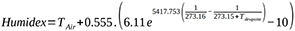
16The Humidex is a function of the dry-bulb temperature and the dew-point temperature. This is a number without a unit, but the Humidex values are close to temperatures in degrees Celsius. This index is calculated as follows (Equation 2):

17Where Tdewpoint and Tair are the temperatures of the dew point and of the air in °C. Note that the exponential multiplied by 6.11 calculates the water vapor pressure (Sahabi-Abed & Kerrouche, 2017).

18The Heat Index is an American index also known as "apparent temperature". This index is calculated as in Equation 3 (NWS, 2022):

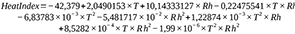
19Where T is the temperature of the dry thermometer (in °F) and where Rh is the relative humidity (in %).

20Since the coefficients presented above (Equation 3) are in degrees Fahrenheit (°F), it is necessary to convert T to°F before calculating the Heat Index. Then we only have to convert the result given by the formula presented in Equation 4. The conversion from Celsius to Fahrenheit is as follows (Equation 4):

21Where TCelsius is the temperature in °C and where TFarenheit is the temperature in °F.

B. Climate modeling

1. The MAR model and its forcings

22The MAR (MAR stands for Modèle Atmosphérique Régional, which means "Regional Atmospheric Model") is a three-dimensional regional climate model developed at ULiège, which is forced to its lateral boundaries by a global climate model or a reanalysis. This model allows, in particular, to physically downscale climate fields at low resolution to simulate climate (by calculating different variables such as temperature, pressure, relative humidity, etc.) over an area of interest with a relatively precise spatial resolution ((Doutreloup et al., 2022). The "downscaling" allows the model to better consider several local atmospheric effects (orography, hydrography, land use, etc.), including the urban heat island effect. This is essential for working on heat waves in a city such as Brussels. For more details on how the MAR works and the MAR simulation analyzed in this study, see Doutreloup et al. (2022).

23For performing future projections, climate simulations from Earth System Models (hereafter ESMs) are used as MAR forcing. An ESM is a numerical global climate model that simulates the Earth’s climate system by representing the atmosphere, oceans, biosphere, cryosphere, and continents (see Gettelman & Rood (2016) for more details). Based on the physical equations contained in the model, an ESM can project climate change according to different SSP (Shared Socioeconomic Pathway) scenarios. Here, we only focus on SSP5-8.5 (Riahi et al. (2017)) often referenced as business as usual. The OCCuPANt dataset provides three simulations of MAR forced by ESMs from the CMIP6 database (Doutreloup et al. (2022)). These three ESMs are BCC-CSM2-MR, MPI-ESM.1.2 and MIROC6. They will be abbreviated by BCC, MPI, and MIR afterward. In addition to these ESMs, which aim to simulate Earth's climate evolution, MAR was forced by the ERA5 reanalysis (representing the observed climate) between 1981 and 2020 for the OCCuPANt project.

24In this study, we consider six periods between 1981 and 2100. These periods are given in Table 1.

Beginning of the period	End of period
1981	2000
2001	2020
2021	2040
2041	2060
2061	2080
2081	2100

Table 2. Periods considered for the study of heat waves between 1981 and 2100.

25The MAR-BCC, MAR-MPI, and MAR-MIR simulations were forced themselves with the SSP5-8.5 scenario for periods in the future (2021 – 2100) and with historical values of greenhouse gas concentrations for periods of the past (1981-2020). For this study, our first task will be to select one of three available global climate models to force MAR. Then, we will analyze and discuss its simulation of the future in terms of heat waves.

26Here, we use periods of the past (1981-2000 and 2001-2020) to evaluate the quality of the different ESMs (downscaled by MAR) by comparing the three ESMs forced reconstructions (MAR-BCC, MAR-MIR, and MAR-MPI) with MAR-ERA5.

27In order to select the most representative ESM, we compare the ability of the three different ESMs to simulate heat waves statistics with respect to the MAR-ERA5 heat waves statistics on the observed past (MAR-ERA5 provides an accurate approximation of the past weather for the studied area). Hence, we implicitly assume that the most appropriate model to simulate the future evolution of heat waves in Brussels with the SSP5-8.5 scenario is the ESM, whose simulation of heat waves between 1981 and 2020 is the closest to MAR-ERA5's heat waves statistics during the same period.

2. The OCCuPANt dataset

28As part of OCCuPANt project (ULiège [OCCuPANt], 2022), this study uses its climatological dataset, produced by Doutreloup & Fettweis (2021), which is in open source license. This dataset consists of .csv files for 12 Belgian cities. This dataset has four files per city, per period, per model (forcing MAR), and per SSP.

29The files were created to comply with ISO 15927-4 (ISO, 2005) in TMY and XMY formats, and the information contained in these four files are:

30• The maximal daily mean temperature (that occurred during a heat wave) simulated by the model;

31• The length of the longest simulated heat wave simulated by the model;

32• The intensity of the most intense heat wave simulated by the model;

33• The number of heat waves simulated by the model during the period.

34• The files containing the number of heat waves simulated by the model during the period also contain the hourly values of thirteen variables for each city and each simulated heat wave day. This is a piece of very precious information. The thirteen values are given in Table 2.

Values	Units
Dry-bulb temperature [°C]	°C
Relative Humidity	%
Global Radiation	W h /m2
Diffuse Radiation	W h /m2
Direct Radiation	W h /m2
Wind Speed	m/s
Dew Point Temperature	°C
Atmospheric Pressure	Pa
Cloudiness	tenths
Sky Temperature	K
Specific Humidity	kg water / kg air

Table 3. Variables for which the model provides hourly values during heat waves.

3. Model comparison methods

35In order to compare the different forcings of MAR (MAR-BCC, MAR-MIR, and MAR-MPI) with MAR-ERA5, we use two methods.

36The first method is to look at the difference between MAR-ERA5 and the other simulations in terms of the different quantities we have listed above (number of heat wave days per period, hottest day temperature, etc.). We represent the gaps between MAR-ERA5 and the models with bar charts.

37The second comparison method (the "histogram method") consists in representing on the same graph two statistical distributions (two histograms with a kernel density estimation curve) to select the most similar distribution to the observed one estimated here by MAR-ERA5 (Timmermans, 2022). In this study, this technique is used to compare MAR-BCC, MAR-MIR, and MAR-MPI's distribution of daily mean temperature during a heat wave with the corresponding distribution of MAR-ERA5. Note that the kernel density estimation curve is generated by a function of the ggplot2 package of the R software.

II. Results and discussion

A. Choice of a climatic model to force MAR

38As mentioned above, we will compare the heat wave simulations of MAR-BCC, MAR-MIR, and MAR-MPI with MAR-ERA5 to select the most performant model and study its simulation of future heat waves in Brussels. This will be done following the two “comparison methods” introduced previously.

39To compare MAR-BCC, MAR-MIR, and MAR-MPI with MAR-ERA5, it is relevant to focus on the gap between the MAR-ESMs heat waves simulations and the MAR-ERA5 ones for basic quantities characterizing a simulation. This is shown in Figure 3 and in Figure 4 for:

40• The number of simulated heat waves during the period;

41• The intensity of the most intense heat wave in the period;

42• The highest simulated temperature;

43• The duration of the longest heat wave;

44• The mean duration of heat waves.

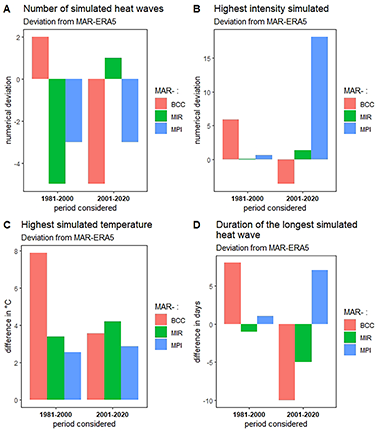
Figure 3. Difference between the ESMs downscaled by the MAR and MAR-ERA5 for the number of simulated heat waves, the greatest simulated intensity, the greatest simulated temperature, and the longest heat wave duration.

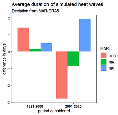
Figure 4. Difference between the ESMs downscaled by the MAR and MAR-ERA5 for the average duration of heat waves.

45In addition, the values associated with MAR-ERA5 (those against which the differences are expressed in Figure 3 and in Figure 4) are given in Table 3.

MAR-ERA5	1981-2000	2001-2020
Number of simulated heat waves	6	10
Highest intensity simulated	5.66	11.73
Highest simulated temperature (°C)	27.21	29.19
Duration of the longest simulated heat wave (days)	8	16
Average duration of simulated heat waves (days)	6.83	8.2

Table 4. MAR-ERA5 values for different quantities of interest in model comparison.

46There is no systematic overestimation or underestimation from MAR-ESMs in terms of the number of simulated heat waves during the two studied reference periods. This is also the case for the highest intensity simulated (except for MAR-MPI), for the duration of the longest heat wave, and for the average duration of the heat waves. Finally, we can observe that all the MAR-ESMs overestimate the highest heat wave temperatures. This should be taken into account when discussing climatic projections.

47On average, while MAR-MIR fails at simulating the number of heat waves in Brussels between 1981 and 2000, it presents the lowest biases on average and then seems to be the most reliable model for simulating the heat waves in the city of Brussels.

48Additionally, the "histogram method", introduced above, can be used in order to decide between the ESMs. The graphs are available in Figure 5 for the period 2001 – 2020 and the dry bulb temperature. Of course, this method can be applied to other cities (i.e., Liège), with other variables (i.e., the dew point temperature), and for other periods (i.e.. 1981-2000).

49By analyzing these graphs, we realize that in addition to the tendency of downscaled global climate models (MAR-BCC, MAR-MIR, and MAR-MPI) to overestimate high temperatures, we notice that the MAR-MIR and MAR-MPI models compare the best with MAR-ERA5.

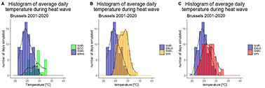
Figure 5. Comparison of the statistical distribution of average daily temperatures during heat waves in Brussels between 2001 and 2020.

50From this study of the reliability of the different models, it emerges that MAR-MIR appears the best relevant among the three available ESMs forced MAR simulation for studying the evolution of heat waves in Brussels in the case of SSP5-8.5.

B. Climate projections

1. Duration and frequency of projected heat waves

51The MAR-MIR simulation was selected to study the evolution of heat waves (projected by the model) for the SSP5-8.5 scenario over the city of Brussels. This Section focuses on the frequency and duration of heat wave events. Regarding the duration of heat waves, Figure 5 reveals that the heat waves simulated in the future are longer than those we currently know.

52Admittedly, it is perfectly logical that the distribution of the duration of heat wave days extends to high values, especially since a heat wave cannot last less than five days, given the definition we have given ourselves. But we do notice some fairly extreme values in Figure 6, including heat waves lasting 40 days or more. In addition to the extreme values, we observe a shift towards higher values of the median heat wave duration during the 21st century, according to MAR-MIR.

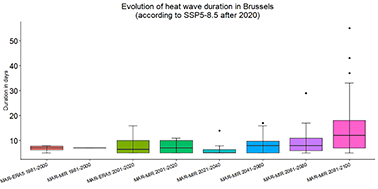
Figure 6. Box plots of heat wave durations according to the period and to the simulation (Note that MAR-ERA5 is abbreviated as MAR-ERA here).

53In addition to the fact that heat waves will be longer in the future, it can be seen in Figure 6 that they will be more frequent. According to MAR-MIR, there will be more and more heat waves over the next decades, independently of the duration of a heat wave. MAR-MIR simulates fewer heat waves between 2021 and 2040 than between 2041 and 2061. Note that Figure 7 shows that there were more heat waves between 2001 and 2020 than between 1981 and 2000 and that, as can be seen in Figure 6, it was longer on average.

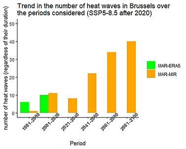
Figure 7. Number of heat waves simulated over the different studied periods.

54Model outputs should be analyzed as climatological data rather than meteorological data. In other words, looking at evolutionary trends rather than one-off events is required. For this reason, a rolling average curve over a five-year window was added to Figure 8, as well as a comparison with MAR-ERA5 allowing us to evaluate of the reliability of MAR-MIR over the current climate. Moreover, Figure 8 highlights the significant interannual variability in climate, so that it does not impact societies in the same way every year or every decade.

55According to the MAR-MIR model, the number of heat wave days per year will increase very strongly in the long term in the SSP5-8.5 greenhouse gas emission scenario, but also that the increase will not occur until 2040 or so as a result of the natural variability in MIROC6 suggesting a break in the temperature increase during the 2020s and 2030s decades.

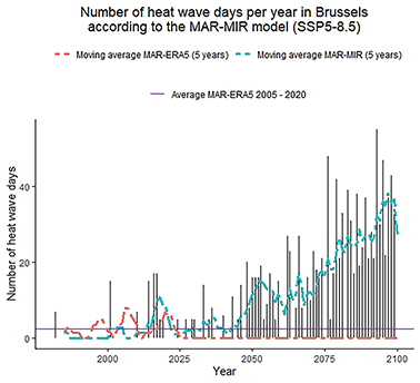
Figure 8. Number of heat wave days per year in Brussels between 1981 and 2100.

2. The intensity of projected heat waves

56In section II.A, the intensity index is introduced to characterize the intensity of a heat wave. It is used here to analyze the evolution of heat waves in Brussels over the 21st century. This index is used here using a graphical representation. Concretely, Figure 9 is strongly inspired by the so-called "bubble" graphs presented in the article on the analysis of heat waves in France by Ouzeau et al. (2016).

57On these graphs, each heat wave is represented by a circle. The surface of the circle is proportional to the intensity of the heat wave. The position of the center of the circle corresponds to the duration of the heat wave in abscissa and to the maximum daily temperature of the heat wave in ordinate. Of course, the color of the “bubbles” corresponds to the period during which the heat wave occurred.

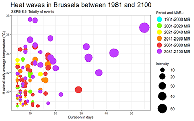
Figure 9. Intensity of heat waves simulated by MAR-MIR in the case of SSP5-8.5 in Brussels by 2100.

a. Nuance for temperature interpretation

58At this stage, it is relevant to state that the maximum temperature simulated by MAR-MIR is generally too high over the current climate (cf. Figure 3), impacting the analysis of the maximum temperature. However, since the definition of intensity depends on thresholds specific to the statistical distributions of the models, the same reasoning should not be applied to absolute temperature as to intensity. Indeed, the definition of this index is independent of a mean bias in maximum temperature, as fixed thresholds will be different for each data set. In other words, any translation of the statistical distribution of average daily temperatures, without a change of variance or any other parameter of this distribution, does not impact the intensity of heat waves.

b. Heat waves in Brussels between 1981-2100

59In Figure 9, the most intense heat waves simulated between now and 2100 are different from those in Brussels in the past. On the one hand, the "small" heat waves of the same type as those experienced by Brussels today during the summer will multiply and become much more frequent. On the other hand, the MAR-MIR simulates much more intense and much warmer heat waves by 2100 following the SSP5-8.5 scenario.

60By way of hypothesis, we can interpret Figure 9 as a move "to higher temperatures" of the local climate temperature distribution. What we call "heat wave" today will be common in 2100 (and even before, of course) while the "real heat wave of the future" will be much more severe (than those of today).

3. Perceived temperature of projected heat waves: Humidex and Heat Index

61Each point corresponds to a heat wave on the graphics shown in Figure 10. Given the scattering of the points making the graph difficult to interpret, LOESS (LOcally Estimated Scatterplot Smoothing) regression curves have been added (see Vaudor (2015) for more details). The graph on the left (A) shows the maximum indices, while the one on the right (B) represents the average indices.

62We can see the average indices' evolution of the mean temperatures is more or less parallel to the evolution of both indexes.

63Regarding the maximum indices, it appears that the temperature indices will more increase than the maximum temperature by 2100.

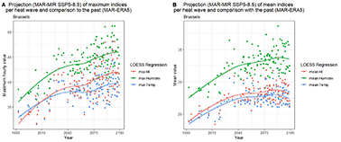
Figure 10. Temperature, heat index (HI), and Humidex average and maximum simulated during heat waves by MAR-MIR in the case of SSP5-8.5 between 1981 and 2100.

64Figure 10 suggests that following our working hypotheses (MAR-MIR in the case of SSP5-8.5), the air will be less supportable during future heat waves than during recent heat waves as temperature indices will increase faster and larger than the maximum temperature.

Conclusion

65This study aimed to characterize the heat waves and predict their future evolution, focusing on Brussels, Belgium. While analyzing the heat wave simulation data in Brussels, it was found that the global climate models downscaled by MAR tend to overestimate the maximum temperatures over the current climate. However, the study results confirmed that the MAR-MIR model was the most robust simulation for predicting the evolution of heat waves in Brussels. The MAR-ERA5 simulations show that the heat waves were more numerous, longer and more intense between 1981 and 2000 than between 2001 and 2020. Based on the SSP5-8.5 climate change scenarios, maximal average daily temperature of heat waves will fluctuate between 32°C and 36°C at the end of this century. In addition, the average duration of heat waves will last between 20 and 30 days (still according to SSP5-8.5). The simulations of heat wave scenarios have shown that if heat waves increase in duration and intensity, causing a climate hazard, future heat waves will be much more problematic if our greenhouse gas emissions evolve according to the SSP5-8.5 scenario, with a projected acceleration of climate change from about 2040. Although climate projections depend on the scenario used, cities and municipalities should start to plan and prepare to mitigate the effects of future heat waves in Brussels and design/retrofit climate-proof buildings. Indoor and outdoor summer thermal comfort conditions are changing (Dartevelle et al., 2022), and there is a serious need for spatial and behavioral adaptation (Attia, 2020).

66To contextualize the study findings, it is important to consider the influence of different climate change scenarios' sensitivity on the results. The climate model implemented in this study used one of the ESMs for the extreme SSP5-8.5 climate change scenario. Three ESMs force the MAR regional model from the CMIP6 database, namely, BCC-CSM2-MR, MPI-ESM.1.2, and MIROC6. Consequently, the results present a highly probable future climate scenario assuming the emissions will not be curbed and business proceeds as usual. The SSP scenario adopted in this study is only dynamically downscaled until the resolution of 5 km resulting in high-resolution generated weather data that are spatially and temporally homogeneous. There are certainly some limitations to the analysis proposed here.

67In the long term, the simulation needs to downscale to lower resolutions up to 1m and create a network of real-time local weather stations that monitors the urban outdoor climate. To analyze these data with greater depth and thus to better understand the projected evolution of our climate, it would be necessary to extend the analysis beyond the thirteen climate variables of this study.

68For example, the influence of humidity and solar radiation on heat wave intensity should be further elaborated. All Belgian cities should be included too. Moreover, a sensitivity analysis should be performed with different climate change scenarios. Despite its relatively small size, Belgium is characterized by fairly interesting climatic variations that we could have studied. In addition to the need to study other cities, other SSPs should certainly be considered using the three ESMs proposed in the database and considering future IPCC scenarios.

69Furthermore, there is a need to develop a common definition of heat waves at the European level to allow the standardization of adaptation and mitigation strategies. The upgrade of building performance requirements and cities towards a climate-resilient and climate-proof built environment is urgent.

70Finally, this study provides novel insights into heat wave characterization and future evolution that can be beneficiary in Belgium and countries with similar temperature climates. We believe the developed methodology can be transferred and applied to other cities worldwide.

Acknowledgements

71The study is part of a wider research project of ULiège, namely OCCuPANt (standing for impacts Of Climate Change on the indoor environmental and energy PerformAnce of buildiNgs in Belgium during summer), which aims to evaluate the impact of climate change on buildings. The project investigates the resilience of the residential building stock against long-term and short-term global warming in Belgian cities (Rahif et al., 2022).

References

72Attia, S. (2020). Spatial and behavioral thermal adaptation in net zero energy buildings: An exploratory investigation. Sustainability, 12(19), 7961. https://doi.org/10.3390/su12197961

73Attia, S., & Gobin, C. (2020). Climate change effects on Belgian households: a case study of a nearly zero energy building. Energies, 13(20), 5357. https://doi.org/10.3390/en13205357

74Bessemoulin, P., Bourdette, N., Courtier, P. & Manach, J. (2004). La canicule d’août 2003 en France et en Europe. La Météorologie, 46, 25 – 33. https://doi.org/10.4267/2042/36057

75Dartevelle, O., Altomonte, S., Masy, G., Mlecnik, E., & Van Moeseke, G. (2022). Indoor Summer Thermal Comfort in a Changing Climate: The Case of a Nearly Zero Energy House in Wallonia (Belgium). Energies, 15(7), 2410. https://doi.org/10.3390/en15072410

76Dobrovolny, P., Moberg, A., Brázdil, R., Pfister, C., Glaser, R., Wilson, R., van Engelen, A., Limanówka, D., Kiss, A., Halícková, M., Macková, J., Riemann, D., Luterbacher & J., Böhm, R. (2010). Monthly, seasonal and annual temperature reconstructions for Central Europe derived from documentary evidence and instrumental records since AD 1500. Climatic Change, 101(1), 69 - 107.

77Doutreloup, S. & Fettweis, X. (2021). Typical & Extreme Meteorological Year and Heat waves for Dynamic Building Simulations in Belgium based on MAR model Simulations. Zenodo. https://doi.org/10.5281/zenodo.5606983.

78Doutreloup, S., Fettweis, X., Rahif, R., El Nagar, E., Pourkiaei, S. M., Amaripadath, D., & Attia, S. (2022). Historical and Future Weather Data for Dynamic Building Simulations in Belgium using the MAR model : Typical & Extreme Meteorological Year and Heat waves. Earth System Science Data, 14(7). https://doi.org/10.5194/essd-2021-401

79Canadian Environmental Service (2018). Aléas météorologiques de la saison chaude. Gouvernement du Canada. https://www.canada.ca/fr/environnement-changement-climatique/services/meteo-saisonniere-dangereuse/aleas-meteorologiques-saison-chaude.html. Consulted on the 10/09/2022.

80García-León, D., Casanueva, A., Standardi, G., Burgstall, A., Flouris, A. D., & Nybo, L. (2021). Current and projected regional economic impacts of heat waves in Europe. Nature communications, 12(1), 1-10. https://doi.org/10.1038/s41467-021-26050-z

81Gettelman, A & Rood, R.B. (2016). Demystifying Climate Models A Users Guide to Earth System Models. Berlin: Springer, 274p. https://doi.org/10.1007/978-3-662-48959-8

82Hémon, D. & Jougla, E. (2004). Surmortalité liée à la canicule d’août 2003 [Rapport remis au Ministre de la Santé et de la Protection Sociale]. INSERM. https://www.inserm.fr/wp-content/uploads/2017-11/inserm-rapportthematique-surmortalitecaniculeaout2003-rapportfinal.pdf. Consulted on the 10/09/2022.

83Hosokawa, Y., Grundstein, .J., Vanos J.K. & Cooper E.R. (2018). Environmental Condition and Monitoring. In Casa, D.J. (ed.) Sport and Physical Activity in the Heat. Cham: Springer, 147 – 162. https://doi.org/10.1007/978-3-319-70217-9

84IPCC, (2022a). Climate Change 2022: Impacts, Adaptation, and Vulnerability. Contribution of Working Group II to the Sixth Assessment Report of the Intergovernmental Panel on Climate Change [H.-O. Pörtner, D.C. Roberts, M. Tignor, E.S. Poloczanska, K. Mintenbeck, A. Alegría, M. Craig, S. Langsdorf, S. Löschke, V. Möller, A. Okem, B. Rama (eds.)]. Cambridge and New York: Cambridge University Press, 3056 p.

85IPCC (2022b). Regional fact sheet - Europe. Intergovernmental Panel on Climate Change. https: //www.ipcc.ch/report/ar6/wg1/downloads/factsheets/IPCC_AR6_WGI_Regional_Fact_She et_Europe.pdf?fbclid=IwAR2XZgccQh-MpaFRNRtPSt-Ol8E3cIS-Fb186bGyR_veLtt_WYDs2eNHsVc. Consulted on the 09/14/2022. 2p.

86IRM (2022). Bilan climatique mensuel – août 2022. Institut Royal Météorologique. https://www.meteo.be/resources/climatology/pdf/bilan_climatique_mensuel_202208.pdf. Consulted on the 09/14/2022.

87ISO (2005). Hygrothermal performance of buildings — Calculation and presentation of climatic data — Part 4: Hourly data for assessing the annual energy use for heating and cooling. International Organization for Standardization. https://www.iso.org/fr/standard/41371.html. Consulted on the 09/01/2022.

88Laaidi, K., Zeghoun, A., Dousset, B., Bretin, P., Vandentorren, S., Giraudet & E., Beaudeau, P. (2012). The Impact of Heat Islands on Mortality in Paris during the 2003 Heat Wave. Environmental Health Perspectives, 120(2) 254 - 259. https://doi.org/10.1289/ehp.1103532

89Larsen, M.A.D., Petrović, S., Radosynski, A.M., McKenna, R. & Balyk, O. (2020). Climate change impacts on trends and extremes in future heating and cooling demands over Europe. Energy and Buildings, 226. https://doi.org/10.1016/j.enbuild.2020.110397

90Macintyre, H. L., Heaviside, C., Taylor, J., Picetti, R., Symonds, P., Cai, X. M., & Vardoulakis, S. (2018). Assessing urban population vulnerability and environmental risks across an urban area during heat waves –Implications for health protection. Science of the total environment, 610, 678-690. https://doi.org/10.1016/j.scitotenv.2017.08.062

91Mastrangelo, G., Fedeli, U., Visentin, C., Milan, G., Fadda, E. & Spolaore, P. (2007). Pattern and determinants of hospitalization during heat waves: An ecologic study. BMC Public Health, 2007, 7, 200. https://doi.org/10.1186/1471-2458-7-200

92Mievis, P. (2020). Bilan de la vague de chaleur d’août 2020. Météo Belgique. https://www.meteobelgique.be/article/nouvelles/la-suite/2418-bilan-de-la-vague-de-chaleur-d-aout-2020. Consulted on the 05/19/2022.

93Ouzeau, G., Soubeyroux, J.-M., Schneider, M., Vautard, R. & Planton, S. (2016). Heat waves analysis over France in present and future climate : Application of a new method on the EURO-CORDEX ensemble. Climate Services, 4, 1 - 12. https://doi.org/10.1016/j.cliser.2016.09.002

94Pascal, M., Wagner, V., Corso, M., Laaidi, K., Ung, A. & Beaudeau, P. (2018). Heat and cold related-mortality in 18 French cities. Environment international, 121(1), 189 – 198. https://doi.org/10.1016/j.envint.2018.08.049

95Patience, G.S. (2013). Temperature. In Patience, G.S. (ed.), Experimental Methods and Instrumentation for Chemical Engineers. Waltham: Elsevier, 145 – 188. https://doi.org/10.1016/B978-0-444-53804-8.00005-8

96Rahif, R., Norouziasas, A., Elnagar, E., Doutreloup, S., Pourkiaei, S. M., Amaripadath, D., ... & Attia, S. (2022). Impact of climate change on nearly zero-energy dwelling in temperate climate: Time-integrated discomfort, HVAC energy performance, and GHG emissions. Building and Environment, 223, 109397. https://doi.org/10.1016/j.buildenv.2022.109397

97Ramon, D., Allacker, K., De Troyer, F., Wouters, H., & van Lipzig, N. P. (2020). Future heating and cooling degree days for Belgium under a high-end climate change scenario. Energy and Buildings, 216, 109935. https://doi.org/10.1016/j.enbuild.2020.109935

98Riahi, K., van Vuuren ,D.P., Kriegler, E., Edmonds, J., O’Neil, B.C., Fujimori, S., Bauer, N., Calvin, K., Dellink, R., Fricko, o., Lutz, W. Popp, A., Crespo Cuaresma, J., KC, S., Leimbach, M., Leiwen, J., Kram, T., Shilpa, R., Emmerling, J.,... Tavoni, M. (2017). The Shared Socioeconomic Pathways and their energy, land use, and greenhouse gas emissions implications : An overview. Global Environmental Change, 42, 153 - 168. https://doi.org/10.1016/j.gloenvcha.2016.05.009

99Sahabi-Abed, S. & Kerrouche, M. (2017). Indices Bioclimatiques : Etude du cas de la Vague de Chaleur en Algérie, Dans la Perspective de l’Elaboration de Cartes de Vigilance : « Humidex » et «PET ». JAMA, 1, 77 – 84. https://www.researchgate.net/publication/324596918_Indices_Bioclimatiques_Etude_du_cas_de_la_Vague_de_Chaleur_en_Algerie_Dans_la_Perspective_de_l’Elaboration_de_Cartes_de_Vigilance_Humidex_et_PET. Consulted on the 05/08/2022.

100Santamouris, M. (2020). Recent progress on urban overheating and heat island research. Integrated assessment of the energy, environmental, vulnerability and health impact. Synergies with the global climate change. Energy and Buildings, 207, 109482. https://doi.org/10.1016/j.enbuild.2019.109482

101Steul, K., Schade, M. & Heudorf, U. (2018). Mortality during heat waves 2003–2015 in Frankfurt-Main – the 2003 heat wave and its implications. International Journal of Hygiene and Environmental Health, 221(1), 81 - 86. https://doi.org/10.1016/j.ijheh.2017.10.005

102Timmermans, G. (2022). L’évolution des canicules à Bruxelles et à Liège sur base du Modèle Atmosphérique Régional (MAR). Travail de fin de bachelier en sciences géographiques, Liège, Université de Liège, inédit, 70p.

103ULiège [OCCuPANt] (2022). OCCuPANt. https://www.occupant.uliege.be/cms/c_7968645/en/occupant. Consulted on the 09/01/2022.

104Van Loenhout, J. A. F., Rodriguez-Llanes, J. M., & Guha-Sapir, D. (2016). Stakeholders’ perception on national heat wave plans and their local implementation in Belgium and the Netherlands. International journal of environmental research and public health, 13(11), 1120. https://doi.org/10.3390/ijerph13111120

105Vandemeulebroucke, I., Caluwaerts, S., & Van Den Bossche, N. (2022). Climate data for hygrothermal simulations of Brussels. Data in brief, 44, 108491. https://doi.org/10.1016/j.dib.2022.108491

106Vaudor, L. (2015). Régression loess. R-atique [server of the individual professional pages of the Ecole Normale Supérieure de Lyon]. http://perso.ens-lyon.fr/lise.vaudor/regression-loess/. Consulted on the 09/05/2022.

107Vautard, R., van Aalst, M., Boucher, O., Drouin, A., Haustein, K., Kreienkamp, F., van Oldenborgh, G.J., Otto, F.E.L., Ribes, A., Robin, Y., Schneider, M., Soubeyroux, J.-M., Stott, P., Seneviratne, S.I., Vogel, M.M. & Wehner, M. (2020). Human contribution to the record-breaking June and July 2019 heat waves in Western Europe. Environmental Research Letters, 15(9). https://doi.org/10.1088/17 48-9326/aba3d4

Pour citer cet article

A propos de : Guillaume TIMMERMANS

A propos de : Sébastien DOUTRELOUP

A propos de : Xavier FETTWEIS

A propos de : Shady ATTIA