Marius LAMBERT, Christoph KITTEL, Adrien DAMSEAUX & Xavier FETTWEIS

Sensitivity of arctic surface temperatures to sea ice thickness changes using the regional climate model mar

Résumé

Depuis le début de ce siècle, l’Océan Arctique a connu une diminution rapide de son étendue de glace de mer, entrainant un réchauffement climatique régional appelé "Amplification Arctique", i.e. deux fois plus marqué que le réchauffement global. En jouant le rôle d’isolant entre l’océan (plus chaud) et l’atmosphère, l’épaisseur et la concentration de glace de mer contrôlent la température à la surface de l’Océan Arctique. Une modification de la température de surface pourrait entrainer une perturbation du système climatique, par le biais de son influence sur la circulation atmosphérique régionale. Dans la plupart des modèles climatiques régionaux (RCMs), la concentration de glace de mer est prescrite par des réanalyses, tandis que l’épaisseur de glace de mer est fixe dans le temps et l’espace, malgré sa variation saisonnière importante. Dans cette étude, on comparera des simulations du MAR forcé par ERA-intérim et OSTIA, i.e utilisant une épaisseur de glace de mer fixe, avec des simulations ou l’épaisseur et la concentration de glace de mer sont prescrites par GLORYS2v4. L’ensemble des simulations concerne le domaine CORDEX-Arctique et couvre la période 2000-2015. L’objectif de ce travail est (i) d’améliorer la représentation de la température de surface, de la vitesse et direction du vent dans la couche limite atmosphérique du MAR en Arctique et; (ii) d’estimer la sensibilité de la température de surface et de la circulation atmosphérique à différentes épaisseurs de glace de mer prescrites dans le MAR. Bien que nous démontrions la sensibilité locale de la température de surface à un changement d’épaisseur de glace de mer (fixe), nous montrons aussi qu’il n’y a pas de bénéfice clair quant à l’utilisation de l’épaisseur de glace de mer variable dans le temps et l’espace comme forçage à la surface du MAR à 50 km de résolution.

Abstract

Since the beginning of this century, the Arctic Ocean has experienced a rapid decrease in sea ice extent, which strongly contributes to a pronounced regional climate warming known as “Arctic Amplification”, i.e. two times as large as the global average. Sea ice concentration (SIC) and sea ice thickness (SIT) mainly control changes in Arctic Ocean surface temperatures by insulating the warmer ocean water from the colder air above. Changes in atmospheric temperatures could perturb the Arctic climate, by affecting the regional atmospheric circulation. In most regional climate models (RCMs), SIC is prescribed from climate reanalyses whereas SIT is fixed in space and time, despite observations of large seasonal variations. Here, we compare climate simulations from the regional climate model MAR forced by the ERA-Interim and OSTIA reanalyses, using fixed SIT, to MAR simulations where SIT and SIC are prescribed by the GLORYS2V4 data set. The set of simulations covers the Arctic-CORDEX domain spanning the whole Arctic Ocean at a spatial resolution of 50 km for the period 2000-2015. This study aims to (1) improve the representation of surface temperatures, wind speed and direction within the Arctic boundary layer simulated by MAR, and to (2) estimate the sensitivity of Arctic surface temperatures and atmospheric circulation to prescribed SIT in MAR. Although our findings highlight the local sensitivity of surface temperatures to SIT changes, they also reveal that there is no clear benefit of using space and time varying SIT data sets to force MAR at 50 km resolution.

Table of content

Introduction

1During the past 50 years, the increase in mean surface air temperature of the Arctic has been twice as large as the global average, a phenomenon called Arctic Amplification (Serreze and Barry, 2011). One of the main causes of Arctic Amplification is considered to be the rapid loss of sea ice (Döscher et al., 2014). Satellite data has shown that sea ice cover decreased by ~4.25 %/decade on average between 1979 and 2015 (Comiso et al., 2017). Measurements of sea ice thickness, although less accurate than of ice extent, have shown a winter decrease of approximately 1.8 m in central Arctic since 1980 (Kwok and Rothrock, 2009; Lindsay and Schweiger, 2015). Of the many mechanisms that accelerate sea ice loss, the sea ice-albedo feedback is one of the most important ones: reduced sea ice extent (SIE) in summer drives increased absorption of solar radiation at the surface of ice free, dark open water. Excess energy retained in ocean water is gradually released during winter, which warms the lower atmosphere and reduces winter sea ice volume. Since this leads to thinner sea ice, it will melt more rapidly in the following summer. This further reinforces ocean warming through enhanced absorption of solar radiation. A second important driver of sea ice loss is the sea ice insulation effect (Serreze and Barry, 2011), which involves sea ice thickness (SIT) rather than SIE. This process is based on the insulating role of sea ice between the ocean and the atmosphere. During winter, ocean heat is transferred through sea ice by conduction towards the colder atmosphere. Thinner sea ice has a lower thermal insulation capacity, which enhances the surface temperature increase. Arctic amplification is stronger in winter and autumn, when the temperature gradient between ocean and lower atmosphere is the largest (Lang et al., 2017). Besides these two main mechanisms, other processes may have partly contributed to recent sea ice decline (e.g. polar clouds radiative forcing (Bennartz et al., 2013; Vavrus, 2004), increased atmospheric water vapor holding capacity (Graversen and Wang, 2009), and recent circulation changes (Overland and Wang, 2016).

2In recent years, there has been a growing attention to Arctic sea ice loss and its impact on climate. However, the focus has been on SIE rather than SIT, despite the fact that the latter plays a key role in the regulation of surface heat fluxes. Until now, due to a lack of reliable data, SIT was often fixed in atmospheric models (Steele and Flato, 2000). However, models with fixed thickness not only tend to underestimate the acceleration of sea ice melt, they also underestimate the warming signal (Lang et al., 2017). Fixed thickness does not take into account the spatial and inter-annual variability of SIT, even though it may induce atmospheric anomalies of almost the same magnitude as those due to a decline in sea ice cover (SIC) (Gerdes, 2006). Rinke et al. (2006) compared their model forced by a fixed 2 m SIT to a regional atmospheric model which was forced by SIT data prescribed by an oceanic model. Results showed that SIT affects the atmospheric circulation and surface temperatures over the whole Arctic Ocean, with the largest changes occurring at the sea ice margins. This is in line with Krinner et al. (2010) who showed that maximum heat transfer takes place at the beginning or end of winter when sea ice is thin and snow cover is shallow. Similarly, Lang et al. (2017) forced a global atmospheric model (EC-earth) with SIT from the assimilation system GIOMAS and compared the simulation to the control run with SIT fixed at 1.5 m. Based on this, Lang et al. (2017) predict a 1ºC increase per decade due to reduced SIT in marginal sea ice areas.

3To improve future projections of Arctic warming, it is crucial to better understand the atmospheric response to sea ice thinning. Here, we use the Modèle Atmosphérique Régional MAR, which is specifically developed to simulate polar climates, to study the impact of prescribed sea ice properties (i.e. SIT, SIC, SST) on Arctic warming and atmospheric circulation.

I. Methods

4This study is part of the CORDEX experiment, since our simulations are on the Arctic-CORDEX domain, i.e. 50 km resolution. The Coordinated Regional Climate Downscaling Experiment (CORDEX) is a double framework initiated in 2009 by the World Climate Research Program (WCRP) (Giorgi et al., 2009).

A. Climate model

5The RCM we used (MARv3.9) is composed of a 3D atmospheric module coupled with a 1D transfer scheme between soil and atmosphere (Soil Ice Snow Vegetation Atmosphere Transfer or SISVAT). The atmospheric part of MAR is described in Gallée and Schayes (1994) and Gallée (1995), while a description of SISVAT can be found in De Ridder and Gallée (1998). The snow-ice part of SISVAT (Gallée and Duynkerke, 1997) is based on the snow model CROCUS developed at the “Centre d’Etudes de la Neige” (CEN) (Brun et al., 1992). Lateral boundaries of MAR are forced every 6 hours depending on a dynamic relaxation procedure (Marbaix et al., 2003). The lateral boundary conditions are surface pressure (SP), temperature (T), two wind components (U and V) and specific humidity (Q) at each vertical level (24 atmospheric layers), as well as SST and SIC above the ocean. Temperature below sea ice is fixed at -2°C and SIT is fixed at 0.5m in the default version of MAR.

B. Data

6Three different reanalyses are used to force MAR (Table 1): (1) the ERA-interim reanalysis of the ECMWF, which was initiated in 2006, and covers the period from 1979 to present, (2) OSTIA, which has been developed by the Met Office of the United Kingdom and provides daily SST and sea ice data at a resolution of 1/20° for the period from 1985 to present, and (3) GLORYS2v4, which is produced by the MyOcean project carried out in the framework of the European Copernicus Marine Environment Monitoring Service (CMEMS) and which provides data (at 1/4°) for the period 1993 to 2015. Note that these three reanalyses are not independent. Since 2009, the SST and SIC that are used to prescribe the ERA-interim model are provided by OSTIA, while GLORYS is based on atmospheric conditions provided by ERA-interim. The default reanalysis which is used to force MAR is ERA-interim.

REANALYSIS	SOURCE	RESOLUTION	TYPE	PERIOD	REFERENCE
ERA-interim	ECMWF	0.75°x0.75°	ATMOSPHERIC	1979-2017	Dee et al. (2011)
OSTIA	NCOF	0.05°x0.05°	OCEANIC	1985-2017	Donlon et al. (2012)
GLORYS2V4	CMEMS / MERCATOR OCEAN	0.25°x0.25°	OCEANIC	1993-2015	Garric et al. (2017)

Table 1. Description of the reanalyses used in this study

C. Experimental setup

7For each simulation of this study (see Table 2), MAR was forced by the ERA-interim reanalysis at its atmospheric lateral boundaries. The simulations differ by the prescribed SIT (0.1, 0.5, 1, 2, 5 or 10 m) and the reanalysis used to force the SIC and SST at the oceanic surface (ERA-interim, OSTIA or GLORYS2v4). The 9 simulations were divided in three groups (MAR-E, MAR-O and MAR-G) depending on the reanalysis used to force SIC and SST in MAR. The reference simulation (MAR-E-0.5) consists of MAR forced by ERA-interim with a SIT fixed at 0.5 m for the period 2000-2016 (Figure 1a). To assess the influence of SIT and SIC on the boundary conditions of MAR over the Arctic, the reference run was compared to 1) five SIT sensitivity experiments (MAR-E-0.1 to MAR-E-10), 2) two SIC and SST sensitivity experiments (MAR-O-0.5 and MAR-G-0.5), and 3) a simulation prescribing spatial and time varying SIT (MAR-G-V).

SIMULATIONS	SIT (m)	FORCING SOURCE AT OCEAN SURFACE
MAR-E-0.5	0.5	ERA-interim
MAR-E-0.1	0.1	ERA-interim
MAR-E-1	1	ERA-interim
MAR-E-2	2	ERA-interim
MAR-E-5	5	ERA-interim
MAR-E-10	10	ERA-interim
MAR-O-0.5	0.5	OSTIA
MAR-G-0.5	0.5	GLORYSv2.4
MAR-G-V	SPATIAL & TIME VARYING	GLORYSv2.4

Table 2. Ensemble of simulations

II. Results

A. Influence of sit

8Figure 1a shows December-January-February (DJF) mean surface temperature from the reference run MAR-E-0.5 for the period 2000-2015. Compared to this reference (Figure 1a), MAR-E-0.1 (Figure 1b) shows a positive anomaly in surface temperature of up to 6ºC near the northern coast of North America, western Russia and over Baffin Bay. This figure illustrates the effect of a thinner sea ice pack (0.1 m) on the temperature rise above sea ice in winter. Figures 1c, 1d, 1e and 1f show the opposite effect, since SIT is fixed at a higher value than in the reference run (Figure 1a). It is shown that, the thicker the sea ice, the stronger the insulation effect, and the colder Arctic surface temperatures. Note the insignificant difference between MAR-E-5 and MAR-E-10 (Figures 1e and 1f). When SIT exceeds 5 m, the atmosphere is strongly buffered from the ocean by the sea ice, which leads to insignificant changes in surface temperature. Finally, Figures 1b, 1c, 1d, 1e, and 1f show a large temperature anomaly due to a change in SIT above the Arctic Ocean, while the anomaly is small above the surrounding continents. In other words, the effect of SIT is mostly local.

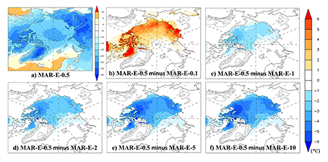
Figure 1. a) Mean surface temperature for DJF modeled by MAR forced by ERA-interim with 0.5 m SIT (MAR-E-0.5) over 2000-2015. b to f) Mean surface temperature anomaly (over ocean and land) for DJF modeled by MAR over 2000-2015. (Hatched = insignificant)

9Figure 2 compares MAR forced by different reanalyses with a fixed SIT (0.5 m). First, the small temperature anomaly displayed in Figure 2a highlights the lack of benefit of using OSTIA instead of ERA-interim reanalysis to force MAR. Despite the high resolution of OSTIA, the differences in surface temperature are sparse and insignificant. Similarly, the benefit of forcing MAR with the intermediate reanalysis GLORYS2v4 is negligible (Figure 2b). Note that the areas with the highest anomalies are common for MAR based on GLORYS and on OSTIA, although anomalies are larger and locally significant for MAR forced by GLORYS. These areas are mainly located at the margins of the sea ice pack: over the Greenland Sea, along the East Asian coast and around the Canadian Archipelago. Surface temperatures in MAR simulations where prescribed SIT is varying in time and space differ significantly from MAR forced by GLORYS with a fixed 0.5 m SIT (Figure 2c). In contrast, simulations MAR-G-V and MAR-E-5 show similar surface temperature patterns (Figures 2c and 1e). This can be explained by the high value of the SIT prescribed in MAR-G-V, which is generally between 3 and 6 meters on average.

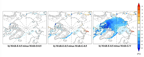
Figure 2. a to c) Mean surface temperature anomaly (over ocean and land) for DJF modeled by MAR over 2000-2015. (Hatched = insignificant)

10Figure 1 and 2 showed the sensitivity of surface temperature to sea ice thickness in winter. Similar figures representing the summer situation (June-July-August) have shown that the temperature anomalies are insignificant in summer (not shown here). This can be explained by the weaker temperature gradient between oceanic waters and the atmosphere during these months.

B. Circulation changes

11Figure 3 shows modeled wind speed and direction. The strongest winds are situated along the coasts of Greenland (~10 m/s), over the North Atlantic (~6 m/s) and locally over most of the coastal regions (~6 m/s) (Figure 3a). Figure 3b shows the small anomaly of wind speed and direction at 8 m height between MAR-E-10 and MAR-E-0.5. Similar results are obtained at altitudes between the surface and 300 hPa. We deduce that SIT does not strongly influence the surface wind pattern for this set-up of MAR at a 50 km resolution.

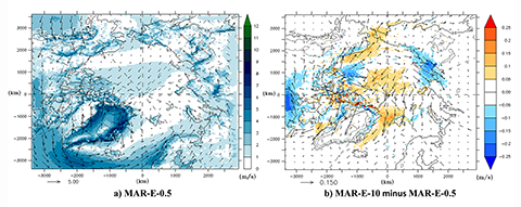
Figure 3. a) Mean wind speed and direction at 8 m height modeled by MAR forced by ERA-interim with SIT=0.5m (MAR-E-0.5) for 2015. b) Mean wind speed and direction anomaly at 8 m height (MAR-E-10 minus MAR-E-0.5) for 2015

III. Discussion and conclusion

12Insignificant and low temperature anomalies were obtained at the margins of the European side of the sea ice pack between MAR-E-0.5 and MAR-E-0.1, 1, 2, 5, 10 (Figures 1b to 1f). However, larger temperature anomalies were expected at the margins of the sea ice pack, where it is relatively thin, than at locations with thick sea ice as reported by Rinke et al. (2006). A plausible reason for this is the influence of surface winds. The spatial variability of wind speed and direction affects the surface temperatures of the Arctic Ocean. If SIT has a greater influence along the northern Russian coast, the North American coast and the isles of the Canadian archipelago, a plausible explanation for this could be the weaker winds observed in these areas and the blocking effect of continents. The blocking effect of continents could also explain a second characteristic visible in Figures 1b to 1f and Figure 2c, which is the minor surface temperature anomaly above continents. This has been confirmed by Deser et al. (2010), who showed that surface air temperature changes are confined under a low-level inversion over the Arctic in winter. Therefore, the air mass influenced by SIT probably does not mix with other air masses above the surrounding continents. As a result, the impact of SIT is only local. Noël et al. (2014) show that the response of the Greenland ice sheet climate to perturbations in SIC and SST is insignificant due to the pronounced katabatic wind blocking effect.

13As shown in Figures 2a and 2b, it turns out that MAR forced by three different reanalyses (ERA-interim, OSTIA and GLORYS2v4) yields similar Arctic surface temperatures. This is not surprising, as these reanalyses are not independent from ERA-Interim. Furthermore, the benefit of using high resolution reanalyses such as GLORYS and OSTIA to prescribe oceanic conditions (SIC, SIT and SST) in MAR is proved insignificant. The reason for this is that we aggregated these reanalyses on the coarse MAR grid at a 50 km spatial resolution. We expect that at a higher resolution (e.g. 10 km), MAR will be able to resolve polynyas, local SST and other small-scale features (Maqueda et al., 2004; Wu et al., 2018).

14To conclude, our results show that the implementation of spatial and time-varying SIT in MAR (i.e. MAR-G-V) is not essential since the surface temperature response to SIT changes in the Arctic Ocean (Figure 2c) does not significantly differ from MAR simulations forced by ERA-Interim with SIT fixed at 2 or 5 m (Figures 1d and 1e). In addition, perturbations in SIT, SIC and SST do not significantly affect the upper atmosphere large-scale circulation since their influence is restricted to the Arctic boundary layer (~100 m) in winter (Jacobson et al., 2000).

References

15Bennartz, R., Shupe, M., Turner, D., Walden, V., Steffen, K., Cox, C., Kulie, M., Miller, N. & Pettersen, C. (2013). July 2012 Greenland melt extent enhanced by low-level liquid clouds. Nature, 496 (7443), 83.

16Brun, E., David, P., Sudul, M. & Brunot, G. (1992). A numerical model to simulate snow-cover stratigraphy for operational avalanche forecasting. Journal of Glaciology, 38 (128), 13-22.

17Comiso, J. C., Meier, W. N. & Gersten, R. (2017). Variability and trends in the arctic sea ice cover: Results from different techniques. Journal of Geophysical Research: Oceans, 122 (8), 6883-6900.

18De Ridder, K. & Gallée, H. (1998). Land surface-induced regional climate change in southern Israel. Journal of applied meteorology, 37 (11), 1470-1485.

19Dee, D. P., Uppala, S., Simmons, A., Berrisford, P., Poli, P., Kobayashi, S., Andrae, U., Balmaseda, M., Balsamo, G., Bauer, d. P. et al. (2011). The era-interim reanalysis: Configuration and performance of the data assimilation system. Quarterly Journal of the royal meteorological society, 137 (656), 553-597.

20Deser, C., Tomas, R., Alexander, M. & Lawrence, D. (2010). The seasonal atmospheric response to projected arctic sea ice loss in the late twenty-first century. Journal of Climate, 23 (2), 333-351.

21Donlon, C. J., Martin, M., Stark, J., Roberts-Jones, J., Fiedler, E. & Wimmer, W. (2012). The operational sea surface temperature and sea ice analysis (ostia) system. Remote Sensing of Environment, 116, 140-158.

22Döscher, R., Vihma, T. & Maksimovich, E. (2014). Recent advances in understanding the arctic climate system state and change from a sea ice perspective: a review. Atmospheric Chemistry and Physics, 14 (24), 13571-13600.

23Gallée, H. (1995). Simulation of the mesocyclonic activity in the Ross Sea, Antarctica. Monthly Weather Review, 123 (7), 2051-2069.

24Gallée, H. & Duynkerke, P. G. (1997). Air-snow interactions and the surface energy and mass balance over the melting zone of west Greenland during the Greenland ice margin experiment. Journal of Geophysical Research: Atmospheres, 102 (D12), 13813-13824.

25Gallée, H. & Schayes, G. (1994). Development of a three-dimensional meso-γprimitive equation model: katabatic winds simulation in the area of terra nova bay, Antarctica. Monthly Weather Review, 122 (4), 671-685.

26Garric, G., Parent, L., Greiner, E., Drévillon, M., Hamon, M., Lellouche, J.-M., Régnier, C., Desportes, C., Le Galloudec, O., Bricaud, C. et al. (2017). Performance and quality assessment of the global ocean eddy-permitting physical reanalysis glorys2v4. In EGU General Assembly Conference Abstracts, volume 19, page 18776.

27Gerdes, R. (2006). Atmospheric response to changes in arctic sea ice thickness. Geophysical Research Letters, 33 (18).

28Giorgi, F., Jones, C., Asrar, G. R., et al. (2009). Addressing climate information needs at the regional level: the cordex framework. World Meteorological Organization (WMO) Bulletin, 58 (3), 175.

29Graversen, R. G. & Wang, M. (2009). Polar amplification in a coupled climate model with locked albedo. Climate Dynamics, 33 (5), 629-643.

30Jacobson, M., Charlson, R. J., Rodhe, H. & Orians, G. H. (2000). Earth System Science: from bio geo-chemical cycles to global changes, volume 72. Academic Press.

31Krinner, G., Rinke, A., Dethloff, K. & Gorodetskaya, I. V. (2010). Impact of prescribed arctic sea ice thickness in simulations of the present and future climate. Climate dynamics, 35 (4), 619-633.

32Kwok, R. & Rothrock, D. (2009). Decline in arctic sea ice thickness from submarine and icesat records: 1958-2008. Geophysical Research Letters, 36 (15).

33Lang, A., Yang, S. & Kaas, E. (2017). Sea ice thickness and recent arctic warming. Geophysical Research Letters, 44 (1), 409-418.

34Lindsay, R. & Schweiger, A. (2015). Arctic sea ice thickness loss determined using subsurface, aircraft, and satellite observations. The Cryosphere, 9 (1), 269-283.

35Maqueda, M. M., Willmott, A. & Biggs, N. (2004). Polynya dynamics: A review of observations and modeling. Reviews of Geophysics, 42 (1).

36Marbaix, P., Gallée, H., Brasseur, O. & van Ypersele, J.-P. (2003). Lateral boundary conditions in regional climate models: a detailed study of the relaxation procedure. Monthly weather review, 131 (3), 461-479.

37Noel, B., Fettweis, X., Van De Berg, W., Van Den Broeke, M. & Erpicum, M. (2014). Sensitivity of Greenland ice sheet surface mass balance to perturbations in sea surface temperature and sea ice cover: a study with the regional climate model mar. Cryosphere (The), 8, 1871-1883.

38Overland, J. E. & Wang, M. (2016). Recent extreme arctic temperatures are due to a split polar vortex. Journal of Climate, 29 (15), 5609-5616.

39Rinke, A., Maslowski, W., Dethloff, K. & Clement, J. (2006). Influence of sea ice on the atmosphere: A study with an arctic atmospheric regional climate model. Journal of Geophysical Research: Atmospheres, 111 (D16).

40Screen, J. A. & Simmonds, I. (2010). The central role of diminishing sea ice in recent arctic temperature amplification. Nature, 464 (7293), 1334.

41Serreze, M. C. & Barry, R. G. (2011). Processes and impacts of arctic amplification: A research synthesis. Global and Planetary Change, 77 (1), 85-96.

42Steele, M. & Flato, G. M. (2000). Sea ice growth, melt, and modeling: A survey. In the fresh water budget of the Arctic Ocean, pages 549-587. Springer.

43Vavrus, S. (2004). The impact of cloud feedbacks on arctic climate under greenhouse forcing. Journal of Climate, 17 (3), 603-615.

44Wu, L., Yang, X.-Y. & Hu, J. (2018). Assessment of arctic sea ice simulations in cmip5 models. Manuscript submitted for publication.

To cite this article

About: Marius LAMBERT

About: Christoph KITTEL

About: Adrien DAMSEAUX

About: Xavier FETTWEIS