


- Accueil
- 78 (2022/1) - De la géomorphologie à la géomatique...
- Assimilation of satellite-derived melt extent increases melt simulated by MAR over the Amundsen sector (West Antarctica)


Visualisation(s): 1657 (27 ULiège)
Téléchargement(s): 86 (1 ULiège)

Assimilation of satellite-derived melt extent increases melt simulated by MAR over the Amundsen sector (West Antarctica)

Document(s) associé(s)
Version PDF originaleRésumé
La fonte de surface sur les plateformes de glace en Antarctique est l'une des plus grandes incertitudes liées à l'augmentation du niveau de la mer pendant le 21e siècle. Cependant, les modèles climatiques actuels peinent encore à la représenter avec précision, ce qui limite la compréhension des processus expliquant sa variabilité spatiale et temporelle et ses conséquences sur la stabilité de l’inlandsis de l’Antarctique. Les progrès récents de surveillance de la Terre grâce aux satellites ont permis de créer de nouvelles estimations de l'étendue de la fonte en Antarctique. Ceux-ci peuvent détecter si et où la fonte se produit, tandis que la quantité d'eau de fonte produite ne peut par contre être déduite que de simulations climatiques. Afin de combiner les avantages des deux outils, nous présentons de nouvelles estimations de la fonte basées sur un modèle climatique régional assimilant l'étendue de la fonte dérivée des satellites. Cela améliore la comparaison entre les estimations du modèle et du satellite, ouvrant ainsi la voie à une ré-estimation de la quantité de fonte produite chaque année à la surface de l'ensemble de l'inlandsis de l’Antarctique.
Abstract
Surface melt over the Antarctic ice shelves is one of the largest uncertainties related to sea level rise over the 21st century. However, current climate models still struggle to accurately represent it, limiting our comprehension of processes driving melt spatial and temporal variability and its consequences on the stability of the Antarctic ice sheet. Recent advances in Earth monitoring thanks to satellites have enabled new estimations of Antarctic melt extent. They can detect if and where melt occurs, while the amount of meltwater produced can only be deduced from model simulations. In order to combine advantages of both tools, we present new melt estimates based on a regional climate model assimilating the satellite-derived melt extent. This improves the comparison between model and satellite estimates paving the way for a re-estimation of the amount of melt produced each year on the surface of the entire Antarctic ice sheet.
Table des matières
Introduction
1The surface melt over the Antarctic ice shelves is an important uncertainty related to projections of sea level rise (SLR) over the 21st century. Although surface melt does not directly contribute to SLR variations as a large part of it is retained by the snowpack and refreezes in place in the following winter, it can have a significant influence on the structure of the Antarctic ice sheet (AIS). Melt water accumulates in ponds on the surface or flows into crevasses flexing and shearing ice shelves that can ultimately trigger their rapid collapse as observed over the northernmost parts of the Antarctic Peninsula (Scambos et al., 2004 ; Vieli et al., 2007 ; Scambos et al., 2009). This process, called hydrofracturing, creates a speed-up in flow (Scambos et al., 2014) of the ice shelves first and subsequently of the upstream grounded glaciers as the ice shelf buttressing is removed (Fürst et al., 2016). This may abruptly accelerate the SLR contribution .
2Despite the risks caused by the presence of liquid water over the ice shelves, melting is still a little known process in Antarctica and surface melt amount estimates remain highly uncertain. For instance, it is not yet clear whether liquid water accumulates on the surface in all parts of Antarctica, or if an organised and large scales drainage system is present, as observed over the Greenland Ice Sheet, reducing the risk of hydrofracturing (Kingslake et al., 2017 ; Dell et al., 2020). This can be partly explained by the restriction of melt production at the margins of the AIS (Arthur et al., 2020), but also by the intrinsic nature of this process whose direct consequence is not directly measurable and as a large part of meltwater is currently retained into the snowpack, thus having no effect on the surface mass balance (SMB) (Agosta et al., 2019). SMB is the balance between accumulation processes at the surface (mainly snowfall) and ablation processes (erosion of snow by the wind, surface sublimation and run-off of melt water).
3Current melt amount estimations rely on local or Antarctic-wide reconstructions by climate models and satellites. Although physically-based climate models generally have biases in their simulations (e.g. Mottram et al., 2021), they directly provide the amount of produced surface melt by representing the surface energy budget and snow properties. This variable is essential to understand which specific conditions result in hydrofracturing (van den Broeke, 2005 ; Lai et al., 2020) and to project the evolution of these conditions in the future (e.g. Donat-Magnin et al., 2021 ; Gilbert & Kittel, 2021). On the other hand, active and passive satellites provide a direct observation of melt since the signal they measure is highly influenced by the presence of liquid water within the snowpack (Zwally. 1977). For instance, tiny amounts of liquid water (less than 1 kg m-2) induce a much higher emissivity than a dry snowpack (Picard et al., 2007 ; Tedesco & Monaghan, 2009 ; Kuipers Munneke et al., 2012 ). Such satellites can detect if and where melt occurs with a small error that only depends on the properties of the surface. The observations are however limited by the revisit time of the satellites, which is at best twice daily (Picard & Filly, 2006). The spatial resolution is in general of the same order of magnitude (or better, Johnson et al., 2020) as the resolution used in the climate models (~ 5 – 30 km). Despite these advantages, the satellites do not detect the amount of meltwater produced, they only provide a binary indicator of the presence or absence of liquid water within the snowpack.
4To better understand the risks of hydrofracturing and associated climate conditions, this is therefore useful to combine both information from models (how much melt) and satellites (where melt actually occurs). This combination is made possible by the assimilation of satellite data into climate models such as reanalyses (e.g. Hersbach et al., 2020). Data from satellites that can be seen as supplementary initial conditions enabling to constrain model estimates in present time. Such an approach has already been used over the Greenland Ice Sheet, for example, and showed reduced bias in model-based simulations (e.g. Navari et al., 2021) but to our knowledge has not yet been applied over the Antarctic ice sheet.
5In this study, we present preliminary results from the polar-oriented regional climate model Modèle Atmosphérique Régional (MAR), developed at the University of Liège, combined with the assimilation of melt detected by satellites over the Amundsen Sea Sector (a region of West Antarctica).
I. Methods
A. The MAR model
6The Modèle Atmosphérique Régional (MAR) is a hydrostatic Regional Climate Model (RCM) whose physical core is described in Gallée and Schayes (1994) and in Gallée (1995) for the hydrometeors (snow particles, cloud ice crystals, rain drops, cloud droplets, and specific humidity). MAR has originally been applied to represent the climate of polar regions, but it has then been adapted to temperate climates such as Belgium (e.g. Wyard et al., 2017 ; Doutreloup et al., 2019).
7MAR physically represents the melt of snow or ice. Its surface module SISVAT (for Soil Ice Snow Vegetation Atmosphere Transfer ; De Ridder, 1997 ; De Ridder & Schayes, 1997 ; Gallée & Duynkerke, 1997 ; Gallée et al., 2001 ; Lefebre et al., 2003) simulates mass and energy transfer between the surface and the atmosphere and in particular explicitly resolves the snow energy budget (SEB). This means that the surface temperature depends on the balance between incoming and out-coming radiative fluxes (shortwave and longwave radiations), turbulent (sensible and latent) heat fluxes and processes such as thermal diffusion, liquid water refreezing or melting. In general, an energy deficit (negative SEB) will result in temperature decrease or liquid water refreezing (if water is present in the snowpack) while an excess in energy (positive SEB) increases the snow temperature and if the snow reaches 0° C, melts it. Surface melt simulated by MAR (version 3.9) has already been compared to satellite data over the Antarctic Ice sheet (e.g. Datta et al., 2019 ; Donat-Magnin et al., 2020). Such comparisons revealed a significant underestimation of surface melt in terms of occurrence and quantity over the Amundsen Sea sector (West Antarctica). Finally, more details about the specific adaptation of MAR v3.11 (version of the model used in this study) for the Antarctic ice sheet can be found in Agosta et al., 2019 and in Kittel et al., 2021.
B. Satellite melt
8The presence of liquid water (i.e. proxy data for surface melt) modifies the brightness temperature (or backscattering coefficient in the case of radar sensors) of the surface which is easily detected (Picard & Fily, 2006). In this study, we use the Advanced Microwave Scanning Radiometer 2 (AMSR2) observations at 18 GHz and horizontal polarisation on board the GCOM-W satellite. The product provides a spatial resolution of 12.5 km that is sufficiently high: 1) to observe melt occurring over marginal areas at the edge of the ice sheet and 2) to compare with climate models. The temporal resolution is daily and is obtained by applying the detection algorithm (see below) on the averaged brightness temperature of all the passes of each day. With at least one satellite observation around local noon everywhere, the product provides an indicator that some melt has occurred in a day. Furthermore, the cold conditions over the Antarctic ice sheet request a high-frequency revisit as they favours sporadic but potentially strong melt events caused by cloud-emitted longwave radiations (e.g. Wille et al., 2019) in addition to the summer events that mainly occur at peak sunshine energy incidence. A discussion about the importance of observational hours can be found in Picard and Fily (2006).
9Melt is detected by the increase in brightness temperature induced by wet snow (> 245 K) compared to dry snow (~ 200 – 220 K). The surface is considered to be melting if the brightness temperature is above a specific threshold. Following the algorithm defined by Torinesi et al. (2003) and improved by Picard and Fily (2006), the threshold is not an absolute value but depends on previous conditions of the snowpack. This enables to take into account the presence of ice layers that alter the brightness temperature of the dry snowpack. In this case, melt is considered to occur if
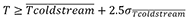
10with T the brightness temperature measure by the sensor, (Formule 2) the mean brightness temperature during the cold season and σ(Formule 3) the standard deviation over the same period.
 (Formule 2)
 (Formule 3)
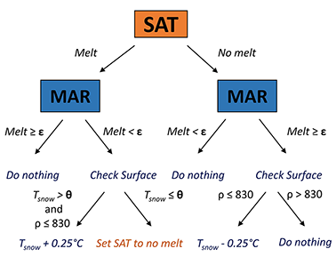
Figure 1. Description of the assimilation routine that is called every model time step between November and March and after 2 h a.m. UTC for each day. ε is the melt threshold at which melting is triggered or stopped in the climate model while θ is a minimum snow temperature under which melt is considered to never occur. ρ refers to the surface density (kg m-3).
C. Assimilation methods and experiments
11The aim of assimilating satellite melt is to constrain / guide the melt production in the surface scheme of MAR during the usual melt season (i.e. November – March). To do so, a binary mask (melt / no melt) is defined following section I.B for each continental Antarctic pixel and for every day. The binary mask has been interpolated to the 12.5 km MAR grid using a simple linear interpolation metric of the four nearest inverse-distance-weighted model grid cells. A satellite pixel is considered as melting if melt extent is > 0.5 after interpolation knowing that it is a binary field (0 – 1) which was interpolated. The assimilation routine is then called each “summer” day at every MAR time step after 2 a.m. (UTC). The short period 0 – 2 a.m. without assimilation enables MAR to balance with its own simulated conditions and to compute a mean liquid water content over a sufficiently large number of time steps without being impacted by assimilation. The assimilation method then distinguishes the cases without and with satellite melt and two subcases depending on MAR internal variables (Figure 1). If the satellite data indicates no melt and MAR has already simulated more melt than a threshold value (ε), then the snow layers up to 1 m below the surface are cooled by 0.25° C until the mean liquid water content (computed from the beginning of the day) does not more reached the threshold value. On the contrary, if there is melt according to the satellite and MAR does not simulate enough melt, the temperature of snow layers up to 1m in depth is increased by 0.25° C. In both cases, if the surface layer is ice (density ρ ≥ 830 kg m-3), the temperature is never changed as MAR prevents liquid water from accumulating in ice layers. If the MAR snow temperature (θ) of the first meter of snow is low (i.e. θ < –7.5° C), it is unlikely that melt occurs and the daily satellite-based binary mask is discarded, thus filtering the probable observation errors. Finally, the two other subcases occur when both MAR and satellite agree with each other and then no changes are made in snow temperature. The threshold for melt (ε) in MAR is set to 0.2 % of liquid water of the first meter snowpack mass averaged since the beginning of the day. This value of liquid water content has been shown to significantly alter the surface brightness temperature measured by satellites (Tedesco et al., 2007). Although the dependence of the MAR results on this threshold remains low (Fig. 2), it will be discussed later in the manuscript (section II).
12In this study, MAR is run at a spatial resolution of 12.5 km similarly to satellite data over the Amundsen Sector region. As it is a regional climate model, MAR is forced by 6-hourly large-scale forcing fields from the ERA5 reanalysis (Hersbach et al., 2020) at its atmospheric lateral boundaries (temperature, specific humidity, wind and pressure), over its oceanic surface (sea ice concentration and sea surface temperature), and at the top of its atmosphere in the stratosphere (wind and temperature). Two simulations are performed: one without assimilating satellite data considered as the reference simulation (MARref) and one with it (MARsat) and are compared hereafter to highlight the interest of assimilating melt extent.
D. The Amundsen Sector region
13The Admunsen Sector, as defined in this study, is a region located in the West AIS (Figure 3c) and includes the western portion of the Ellsworth Land and the eastern portion of the Marie Byrd Land. As on most of the margins of the AIS, the grounded-originating ice flows over the ocean creating large (> 100 km) ice shelves. Surface elevation ranges from ~ 0 m over the ice shelves up to 2 300 m over the high plateau and nunatak summits. The region is strongly affected by climate change and accounts for 60% of the Antarctic mass loss (Rignot et al., 2019). In particular, the loss of ice shelf buttressing caused by basal (i.e. ocean) melt has lead to ice thickness decrease with further potential strong consequences on the stability of the West AIS. The Admunsen Sector is characterised by a retrograde bedrock slope enabling warm water to penetrate further beneath the ice and increasing melt triggering positive feedbacks that can lead to the collapse of the West AIS (Pattyn et al., 2018).
14Although the surface melt amount is not so frequent than over the Antarctic Peninsula, strong melt events can be caused by atmospheric blocking conditions (Wille et al., 2019). Surface melt (in addition to the effects of glacial dynamics) over this region could then contribute to damage the ice shelves (Lhermitte et al., 2020). The amount of surface melt over the Amundsen region is still little known as a consequence of important biases in climate models likely due to the heterogeneous relief combined with the periodic and not widespread occurrence of melt (Donat-Magnin et al., 2020). This makes the Amundsen Sector an interesting region to develop an assimilation method that should reduce model biases to improve our comprehension of processes leading to ice shelf damages with further consequences on the stability of the West AIS.
II. Results
A. Evaluation against weather observations
15Before analysing the effect of the assimilation on the simulated melt, we evaluate MAR near-surface climate against near-surface temperature and wind observations from Automatic Weather Station (AWS) located in our area of interest – see figure 3 for the locations of the AWS and Kittel et al. (2021) for the comparison methodology. We only show the values for MARref in table 1 because we found that the comparison statistics are the same for both simulations. This means that corrections related to satellite derived melt extent only affect the snowpack conditions and sub-surface melt in MAR, but not the near-surface atmosphere.
|
Mean bias |
RMSE |
CRMSE |
Correlation |
|
|
Near-surface temperature (° C) |
+ 0.2 |
1.7 |
1.7 |
0.91 |
|
Near-surface wind speed (m s-1) |
– 1.2 (6.0 ± 3.1) |
2.1 |
2.1 |
0.85 |
Table 1. Comparison between the MAR simulation without assimilation (MARref) and in situ observations in summer (DJF). The mean bias (° C or m s-1), the Root Mean Squared Error (RMSE, ° C or m s-1), the centred Root Mean Squared Error (CRMSE, ° C or m s-1), and the correlation are listed. CRMSE is the RMSE where systematic biases (notably due to elevation differences) have been removed. The mean observed value and standard deviation are listed in brackets in the mean bias columns. The simulation with assimilation has exactly the same statistics (not shown).
16The evaluation reveals a correct representation of the near-surface climate. The small temperature overestimation is considered to be non-significant compared to the cold temperature over the Amundsen sector. Finally, we note a (still not statistically significant) underestimation of near-surface wind speed likely due to the relatively coarse simulation resolution used here. Katabatic wind speed is underestimated due to the smoothed topography since this kind of wind is enhanced by slope and channeling in valleys. Furthermore, the majority of the biases are due to a single station (Toney Mountain, see figure 3 for the localisation) potentially suggesting measurement errors.
B. Evaluation of melt extent against satellite melt
17
Assimilating satellite melt extent in MAR improves the representation of the melt extent over the Amundsen Sector (Figure 2). Melt extent in MAR is defined as the fraction of the domain where the daily mean liquid water content over the first meter of the snowpack is at least equal to 0.2 %. However, accounting for this only threshold in liquid water content would not enable a fair comparison in presence of blue ice at the surface as the MAR retention scheme snow model does not enable to retain water in the presence of ice because no pore space is available. Locations where the surface snow density is higher than 830 kg m-3 (Harper et al., 2012) are then considered as melting in addition to pixels reaching the liquid water content threshold. Note that using a different threshold – 0.1 % to 0.3 % – does not change the comparison as shown in figure 2. Although the reference simulation already has a fairly correct representation of the melt extent, figure 2 reveals some improvements in MARsat for both small events (including the ones at the beginning and end of the melt season, see 2013) or some major events (e.g. in 2017). Furthermore, the end of the melt season is also better simulated as in 2016. Despite significant improvements, exceptions can occur notably in late March 2015 when MARsat overestimates the peak of melt.
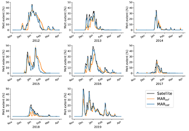
Figure 2. Evolution of the daily melt extent (in % of the MAR integration domain) in summer (2013 – 2020) from satellite observations (blue), and as simulated by MAR (without assimilation, i.e. MARref, in black and with assimilation, i.e. MARsat, in red). MAR melt extent is computed as the fraction of the domain where the liquid water content of the snowpack is at least equal to 0.2 % (sensitivity from 0.1 to 0.3 % of this threshold is shown with grey shading MARref ).
C. Spatial comparisons
18The following analysis focuses on spatial evaluation, starting with the comparisons between the melt extent from satellite and from the reference simulation (MARref) before discussing improvements when using the assimilation (MARsat). We conclude by discussing the remaining biases and potential causes.
19As highlighted by figure 3, MARref underestimates the melt days over the Amundsen sector. Both the extension and the magnitude are underestimated. The satellite detects many more melt days, especially over ice shelves surrounded by complex topographic features (Abbot and Cosson) in the easternmost part of the domain. This can be related to the too coarse resolution in MAR preventing a correct representation of processes leading to melt in such areas as adiabatic warming due to katabatic winds or cloud-orography interactions. Over these ice shelves, the satellite detects up to 20 more melt days than MARref, explaining the underestimation of melt days. According to the satellite, melt can also periodically occur over high altitude locations (even higher than 1 500 m) while melt is limited below 500 m above sea level in MARref. This therefore questions the satellite reliability over these high altitude areas as the air temperature over these locations is supposed to remain very low (AWS data or MAR suggest maximum air temperature below –2° C).
20On the opposite, MARref simulates more melt days over some local areas (Figure 3). This is notably the case over the Getz Ice Shelf (located on the westernmost part of the domain) that is more widespread and surrounded by a flatter environment. MARref also simulates more melt over the edge of the Abbot Ice shelf that could either result from too warm sea surface conditions leading to melt in the model or an underestimation of the satellite due to mixing signals between sea ice and the ice shelf (microwave antenna sidelobes). Finally, note the presence of a small area close to the Cosgrove Ice Shelf with a significant overestimation in MAR. In this area, MAR suggests the presence of blue ice on the surface. The number of actual melt days (i.e. where meltwater is produced) simulated by MAR remains lower (on average less than 10 days per summer) than the number of MAR melt days computed using ε larger than 0.2 % and including blue ice areas (on average more than 50 days per summer). It is very likely that the disagreement in this area between MAR and satellite results mainly from an artefact in our melt detection in both MAR and satellite as we consider blue ice in MAR as melting even if it might be not the case and the satellite signal is also perturbed by the presence of ice on the surface (Fettweis et al., 2007).
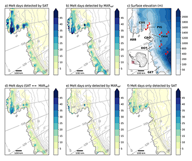
Figure 3. Top: Mean number of melt days over the 2012 2019 summers from satellite (a) and as simulated by MAR without assimilation (b). MAR surface elevation (m above sea level) of the Amundsen Sector with an insert locating this region (red) in Antarctica. Red numbers correspond to AWS locations used to evaluate MAR (1: Evans Knoll ; 2: Backer Island ; 3: Kohler Glacier ; 4: Lower Thwaites Glacier ; 5: Toney Mountain ; 6: Up Thwaites Glacier). Major and discussed ice shelves are also located: Abbot (ABB) ; Cosgrove (COS) ; Pine Island Glacier (PIG) ; Thwaites (THW) ; Dotson (DOT) ; Crosson (CRO) and Getz (GET). Below: Number of melt days where both MARref and the satellite suggest melt (d), where only MARref suggests melt (d), and only the satellite detects melt (f). A melt day in MARref is defined as a day where the mean liquid water content of the snowpack is at least equal to 0.2 %, and also where snow density is higher than 830 kg m-3.
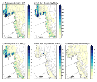
Figure 4. Same as figure 3 but with MARSAT where satellite melt extent has been assimilated into. Top: melt days using satellite detection (a) and simulated by MARsat (b). Below: number of melt days where both MARsat and the satellite suggest melt (c), where only MARsat suggests melt (d), and only the satellite detects melt (e) at the surface. A melt day in MARsat is defined as a day where the liquid water content of the snowpack is at least equal to 2 %, and also where snow density is higher than 830 kg m-3.
21The assimilation of melt extent reduces the discrepancies between MAR and the satellite. This leads to an increase in the number of melt days simulated by MARsat over both coastal areas and locations below 1 000 m above sea level. Most importantly, the number of melt days where both are in agreement is higher in particular by a reduction of days where only the satellite detects melt (Figure 4). The assimilation also prevents MARsat from simulating its own events by inhibiting melt production in the model when the satellite does not detect it. Note that the overestimation of melt days by MAR shown in figure 4d only results from the artefact in the comparison and the presence of blue ice at the surface in MAR. The presence of blue ice in these regions is not only created by melt but also by the removal of snow precipitation by the strong katabatic winds (sublimation and erosion).
22However despite this overall improvements,, the satellite still suggests locally melt that is not represented in MARsat. Over high locations, MARsat snow temperature remains too low (below –7.5° C) so that the assimilation scheme has been disabled. The same reason explains the remaining differences over the Abbot, Cosgrove and edge of Pine Islands ice shelves. As mentioned before, MAR can underestimate the temperature over these areas by underestimating the adiabatic warming resulting from the compression of katabatic winds. In this case, the temperature condition (θ) would wrongly prevent melt. Another possibility is an error from the satellite that would detect excessive melting of the surface while production of melt water does actually not occur. MAR suggests that these areas are made of blue ice, i.e. with a low albedo and higher surface density contrasting with other regions in this sector where the surface is made of snow (Figure 5). High-density snow leads to a decrease of the brightness temperature, an effect on the signal similar to the dry snowpack. This comparison reveals important discrepancies between the model and the satellite due to the presence of blue ice.
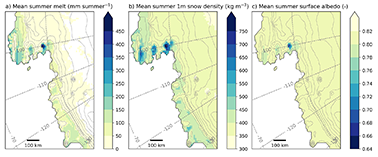
Figure 5. Mean summer cumulated melt water production (mm summer-1), snow density over the first meter of snow (kg m-3), and surface albedo (-) as simulated by MARsat over 2013 – 2020.
D. Impacts of the assimilation on water production
23The assimilation of satellite detection enhances more meltwater production associated with the increase in melt days. Locally, MARsat simulates more melt up to 300 mm summer-1 compared to MARref (Figure 5) and by ~ 27 % over the whole domain (Table 2), although this remains lower than the inter-annual variability and is therefore considered as non-significant. This increase in melt is also translated into higher snow densities reducing the pore volume of the firn and then the MAR meltwater retention capacity. As the pore volume decreases, liquid water can no longer percolate as easily through the firn where it can refreeze, but tends to saturate the snowpack leading to more (+ 175 %) water run-off (Table 2). Since the atmospheric properties and snowfall remain unchanged, higher run-off values reduce the SMB over the Amundsen Sector (Table 2). Note however that changes in ablation by run-off remain low compared to the accumulation by snowfall so that the changes in SMB can be considered here as negligible, meaning no direct impact to the SLR. While previous studies (e.g. Kittel et al., 2021) have suggested that MAR tends to simulate more surface melt and mass loss by meltwater run-off compared to other state-of-the-art climate models over the Antarctic ice sheet, this study suggests that this quantity may still be underestimated even in MAR.
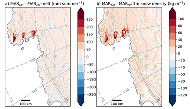
Figure 6. Anomaly of mean cumulated summer melt (mm yr-1) and snow density over the first meter of snow (kg m-3) simulated by MARsat compared to MARref over 2013 – 2020.
III. Discussion
|
SMB (Gt summer-1) |
Melt (Gt summer -1) |
Run-off (Gt summer-1) |
1m Snow density (kg m-3) |
||
|
MARref |
103.5 ± 24.9 |
14.9 ± 8.5 |
0.8 ± 0.6 |
391.1 ± 4.6 |
|
|
MARsat-0.2%-7.5°C |
1.4 |
+4.1 |
+1.4 |
+4.1 |
|
|
MARsat-0.1%-7.5°C |
0.8 |
+2.3 |
+0.8 |
+2.6 |
|
|
MARsat-0.3%-7.5°C |
1.1 |
+4.1 |
+1.4 |
+4.0 |
|
|
MARsat-0.2%-5°C |
1.5 |
+4.6 |
+1.8 |
+4.0 |
|
|
MARsat-0.2%-3°C |
1.3 |
+5.1 |
+1.2 |
+5.2 |
|
Table 2. Mean summer Surface Mass Balance (Net snow accumulation, i.e. snowfall run-off sublimation) (Gt summer-1, i.e. 109 t summer-1) , melt (Gt summer-1), and run-off (Gt summer-1) integrated over the whole domain, as well as first meter depth snow mean density (kg m-3 ) and temperature (° C) averaged over the whole domain. Values for the simulation with different assimilation methods are given in anomalies using the simulation without any assimilation (MARref) as a reference. MARsat-0.2%-7.5°C is the reference assimilation simulation called MARsat so far.
24The assimilation method either triggers melting by warming the snowpack if MAR does not simulate any, or conversely inhibits melting by cooling if MAR simulates too much. The not enough / too much threshold is set to a value of 0.2 % of liquid water in the snowpack to be coherent with the amount of liquid water that alters the brightness temperature measured by satellites. However, uncertainties remain about the exact values as the presence of a tiny amount of liquid water can already change the brightness temperature as highlighted by Tedesco et al. (2007). Furthermore, the satellite data is set to “no melt” to prevent MAR from generating melt where surface conditions are considered as too cold (–7.5° C).
25We will then discuss the sensitivity of the results to these factors. With this in mind, we carried out different sensitivity experiments where the melting threshold (0.1 % and 0.3 %) and the minimum temperature at which assimilated melting is allowed to occur (–5° C and –3° C) were changed. In all the experiments, melt (and also run-off) is found to increase by ~ 15 % to ~ 34 % compared to MARref (Table 2). Using a small threshold (ε = 0.1 %) for assimilating melt leads to a lower increase in melt as it strongly inhibits MAR to generate its own event, although the differences remain negligible. A higher threshold (ε = 0.3 %) does not change the results. As for the minimum temperature threshold (θ), enabling the assimilation to occur at higher temperature (θ = –5° C and θ = –3° C) leads to similar results (Table 2). This suggests that results are not influenced by the liquid water threshold (ε), nor by the threshold temperature (θ) that are defined to trigger or inhibit melt.
Conclusions
26In the previous sections, we showed the interest of assimilating melt detected by microwave satellites in MAR to generate new melt estimates. Such estimates benefit from the advantages of the two products as satellites indicate whether the surface is melting or not with a high confidence, while MAR quantifies the intensity of the melt but can be cold or warm biased. Triggering or inhibiting melt in the model given observations improves the comparison of MAR results with the observations, showing that the data assimilation is active.
27However, these benefits are discussed by a comparison with the same product as used in the data assimilation so that the evaluation is not independent. Further work will then consist in comparing the new MAR simulations using other satellite products as QuikSCAT (e.g. Steiner & Tedesco, 2014) or synthetic aperture radar (SAR) images (e.g. Johnson et al., 2020) to confirm the better representation of surface and sub-surface melt in MAR. Using independent products could improve our comparison but Datta et al. (2018) found uncertainties in melt detection between different satellite products as large as the ones found in this study between MAR and AMSR2. Another possibility could also be to create a binary mask of melt detected not only by AMR2 but also by other satellite products to reduce the observational errors.
28Furthermore, our results have also revealed a strong disagreement between satellite and MAR over blue ice areas or in high-elevation areas that could question the reliability of melt detection based on brightness temperature. Blue ice areas are a common feature of the Antarctic ice sheet as the strong katabatic winds enhance the removal of snow by erosion and sublimation. These areas are essentially located over the margins of the ice sheet where the adiabatic compression of katabatic winds dries out the air mass (promoting sublimation) and where the winds are strong enough to erode the surface (i.e. where the slope is steep). These interactions between winds and surface have been shown to promote melt near the grounding line and over ice shelves (Lenaerts et al., 2017) with the possible consequence of increasing the risk of hydrofracturing. This notably highlights the importance of the proper melt detection by satellites and their adequate representation in climate models.
29The preliminary results presented in this study stresses the need of applying the assimilation method over the whole Antarctic ice sheet instead of a small region of the Amundsen Sector. While AWS air temperature compares well with MAR, assimilating the satellite detection in MAR leads to an increase in surface melt and run-off. This could revise melt estimates and our current comprehension of the ice sheet dynamics and risk of hydrofracturing. Furthermore, these new results could provide better estimates of firn density (that is sensitive to melt). It will help to reduce uncertainties in elevation changes deduced from satellites (e.g. Helsen et al., 2008) and then contribute to better estimation of recent Antarctic mass changes and contribution to sea level rise.
References
30Agosta, C., Amory, C., Kittel, C., Orsi, A., Favier, V., Gallée, H., van den Broeke, M.R., Lenaerts, J., van Wessem, J. M., van de Berg, W.J. & Fettweis, X. (2019). Estimation of the Antarctic surface mass balance using the regional climate model MAR (1979-2015) and identification of dominant processes. The Cryosphere, 13, 281-296. https://doi.org/10.5194/tc-13-281-2019
31Arthur, J.F., Stokes, C., Jamieson, S.S., Carr, J.R. & Leeson, A.A. (2020). Recent understanding of Antarctic supraglacial lakes using satellite remote sensing. Progress in Physical Geography: Earth and Environment, 0309133320916114. https://doi.org/10.1177%2F0309133320916114
32Datta, R.T., Tedesco, M., Agosta, C., Fettweis, X., Kuipers Munneke, P. & Broeke, M.R. (2018). Melting over the northeast Antarctic Peninsula (1999–2009): evaluation of a high-resolution regional climate model. The Cryosphere, 12, 2901-2922. https://doi.org/10.5194/tc-12-2901-2018
33Datta, R.T., Tedesco, M., Fettweis, X., Agosta, C., Lhermitte, S., Lenaerts, J.T. & Wever, N. (2019). The effect of Foehn-induced surface melt on firn evolution over the northeast Antarctic peninsula. Geophysical Research Letters, 46, 3822-3831. https://doi.org/10.1029/2018GL080845
34De Ridder, K. (1997). Radiative transfer in the IAGL land surface model. Journal of Applied Meteorology, 36, 12-21. https://doi.org/10.1175/1520-0450(1997)036%3C0012:RTITIL%3E2.0.CO;2
35De Ridder, K. & Schayes, G. (1997). The IAGL land surface model. Journal of applied meteorology, 36, 167-182. https://doi.org/10.1175/1520-0450(1997)036%3C0167:TILSM%3E2.0.CO;2
36Dell, R., Arnold, N., Willis, I., Banwell, A., Williamson, A., Pritchard, H. & Orr, A. (2020). Lateral meltwater transfer across an Antarctic ice shelf. The Cryosphere, 14, 2313-2330. https://doi.org/10.5194/tc-14-2313-2020
37Donat-Magnin, M., Jourdain, N.C., Gallée, H., Amory, C., Kittel, C., Fettweis, X., Wille, J.D., Favier,V., Drira, A. & Agosta, C. (2020). Interannual variability of summer surface mass balance and surface melting in the Amundsen sector, West Antarctica. The Cryosphere, 14, 229-249. https://doi.org/10.5194/tc-14-229-2020
38Donat-Magnin, M., Jourdain, N.C., Kittel, C., Agosta, C., Amory, C., Gallée, H., Krinner, G. & Chekki, M. (2021). Future surface mass balance and surface melt in the Amundsen sector of the West Antarctic Ice Sheet. The Cryosphere, 15, 571-593. https://doi.org/10.5194/tc-15-571-2021
39Doutreloup, S., Kittel, C., Wyard, C., Belleflamme, A., Amory, C., Erpicum, M. & Fettweis, X. (2019). Precipitation evolution over Belgium by 2100 and sensitivity to convective schemes using the regional climate model MAR. Atmosphere, 10, 321. https://doi.org/10.3390/atmos10060321
40Fettweis, X., van Ypersele, J.-P., Gallée, H., Lefebre, F. & Lefebvre, W. (2007). The 1979–2005 Greenland ice sheet melt extent from passive microwave data using an improved version of the melt retrieval XPGR algorithm. Geophysical Research Letters, 34, L05502. https://doi:10.1029/2006GL028787
41Fürst, J.J., Durand, G., Gillet-Chaulet, F., Tavard, L., Rankl, M., Braun, M. & Gagliardini, O. (2016). The safety band of Antarctic ice shelves. Nature Climate Change, 6, 479-482. https://doi.org/10.1038/nclimate2912
42Gallée, H. (1995). Simulation of the mesocyclonic activity in the Ross Sea, Antarctica. Monthly Weather Review, 123, 2051-2069. https://doi.org/10.1175/1520-0493(1995)123%3C2051:SOTMAI%3E2.0.CO;2
43Gallée, H. & Duynkerke, P.G. (1997). Air-snow interactions and the surface energy and mass balance over the melting zone of west Greenland during the Greenland Ice Margin Experiment. Journal of Geophysical Research: Atmospheres, 102, 13 813-13 824. https://doi.org/10.1029/96JD03358
44Gallée, H., Guyomarc’h, G. & Brun, E. (2001). Impact of snow drift on the Antarctic Ice Sheet surface mass balance: Possible sensitivity to snow-surface properties. Boundary-Layer Meteorology, 99, 1-19. https://doi.org/10.1023/A:1018776422809
45Gallée, H. & Schayes, G. (1994). Development of a three-dimensional meso-γprimitive equation model: katabatic winds simulation in the area of Terra Nova Bay, Antarctica. Monthly Weather Review, 122, 671-685. https://doi.org/10.1175/1520-0493(1994)122<0671:DOATDM>2.0.CO;2
46Gilbert, E. & Kittel, C. (2021). Surface Melt and Runoff on Antarctic Ice Shelves at 1.5° C, 2° C, and 4° C of Future Warming. Geophysical Research Letters, 48, e2020GL091 733. https://doi.org/10.1029/2020GL091733
47Harper, J., Humphrey, N. & Pfeffer, W. (2012). Greenland ice-sheet contribution to sea-level rise buffered by meltwater storage in firn. Nature, 491, 240-243. https://doi.org/10.1038/nature11566, 2012
48Helsen, M.M., Van Den Broeke, M.R., Van De Wal, R.S., Van De Berg, W.J., Van Meijgaard, E., Davis, C.H., Li, Y. & Goodwin, I. (2008). Elevation changes in Antarctica mainly determined by accumulation variability. Science, 320, 1626-1629. https://doi.org/10.1126/science.1153894
49Hersbach, H., Bell, B., Berrisford, P., Hirahara, S., Horányi, A., Muñoz-Sabater, J., Nicolas, J., Peubey, C., Radu, R., Schepers, D., Simmons, A., Soci, C., Abdalla, S., Abellan, X., Balsamo, G., Bechtold, P., Biavati, G., Bidlot, J., Bonavita, M., De Chiara, G., Dahlgren, P., Dee, D., Diamantakis, M., Dragani, R., Flemming, J., Forbes, R., Fuentes, M., Geer, A., Haimberger, L., Healy, S., Hogan, R.J., Hólm, E., Janisková, M., Keeley, S., Laloyaux, P., Lopez, P., Lupu, C., Radnoti, G., de Rosnay, P., Rozum, I., Vamborg, F., Villaume, S. & Thépaut, J.-N. (2020). The ERA5 global reanalysis. Quaterly Journal of the Royal Meteorologic Society, 146, 1999-2049. https://doi.org/10.1002/qj.3803
50Johnson, A., Fahnestock, M. & Hock, R. (2020). Evaluation of passive microwave melt detection methods on Antarctic Peninsula ice shelves using time series of Sentinel-1 SAR. Remote Sensing of Environment, 250, 112 044. https://doi.org/10.1016/j.rse.2020.112044
51Kingslake, J., Ely, J.C., Das, I. & Bell, R.E. (2017). Widespread movement of meltwater onto and across Antarctic ice shelves. Nature, 544, 349-352. https://doi.org/10.1038/nature22049
52Kittel, C., Amory, C., Agosta, C., Jourdain, N.C., Hofer, S., Delhasse, A., Doutreloup, S., Huot, P.-V., Lang, C., Fichefet, T. & Fettweis, X. (2021). Diverging future surface mass balance between the Antarctic ice shelves and grounded ice sheet. The Cryosphere, 15, 1215-1236. https://doi.org/10.5194/tc-15-1215-2021
53Kuipers Munneke, P., Van den Broeke, M., King, J., Gray, T. & Reijmer, C. (2012). Near-surface climate and surface energy budget of Larsen C ice shelf, Antarctic Peninsula. The Cryosphere, 6, 353-363. https://doi.org/10.5194/tc-6-353-2012
54Lai, C.-Y., Kingslake, J., Wearing, M.G., Chen, P.-H.C., Gentine, P., Li, H., Spergel, J.J. & van Wessem, J.M. (2020). Vulnerability of Antarctica’s ice shelves to meltwater-driven fracture. Nature, 584, 574-578. https://doi.org/10.1038/s41586-020-2627-8
55Lefebre, F., Gallée, H., van Ypersele, J.-P. & Greuell, W. (2003). Modeling of snow and ice melt at ETH Camp (West Greenland): A study of surface albedo. Journal of Geophysical Research: Atmospheres, 108, 4231. https://doi.org/10.1029/2001JD001160
56Lenaerts, J., Lhermitte, S., Drews, R., Ligtenberg, S., Berger, S., Helm, V., Smeets, C., Van Den Broeke, M., Van De Berg, W.J., Van Meijgaard, E., Eijkelboom, M. & Pattyn, F. (2017). Meltwater produced by wind–albedo interaction stored in an East Antarctic ice shelf, Nature climate change, 7, 58-62. https://doi.org/10.1038/nclimate3180
57Lhermitte, S., Sun, S., Shuman, C., Wouters, B., Pattyn, F., Wuite, J., Berthier, E. & Nagler, T. (2020). Damage accelerates ice shelf instability and mass loss in Amundsen Sea Embayment. Proceedings of the National Academy of Sciences of the USA, 117(40), 24735-24741. https://doi.org/10.1073/pnas.1912890117
58Mottram, R., Hansen, N., Kittel, C., van Wessem, J. M., Agosta, C., Amory, C., Boberg, F., van de Berg, W. J., Fettweis, X., Gossart, A.,van Lipzig, N.P.M., van Meijgaard, E., Orr, A., Phillips, T., Webster, S., Simonsen, S.B. & Souverijns, N. (2021). What is the surface mass balance of Antarctica? An intercomparison of regional climate model estimates. The Cryosphere, 15, 3751-3784. https://doi.org/10.5194/tc-15-3751-2021
59Navari, M., Margulis, S.A., Tedesco, M., Fettweis, X. & van de Wal, R.S. (2021). Reanalysis Surface Mass Balance of the Greenland Ice Sheet along K-transect (2000-2014). Geophysical Research Letters, e2021GL094602. https://doi.org/10.1029/2021GL094602
60Pattyn, F., Ritz, C., Hanna, E., Asay-Davis, X., DeConto, R., Durand, G., Favier, L., Fettweis, X., Goelzer, H., Golledge, N.R., Kuipers Munneke, P., Lenaerts, J.T.M., Nowicki, S., Payne, A.K., Robinson, A., Seroussi, H., Trusel, L.D. & van den Broeke, M. (2018). The Greenland and Antarctic ice sheets under 1.5° C global warming. Nature Climate Change, 8, 1053-1061. https://doi.org/10.1038/s41558-018-0305-8
61Picard, G. & Fily, M. (2006). Surface melting observations in Antarctica by microwave radiometers: Correcting 26-year time series from changes in acquisition hours. Remote sensing of environment, 104, 325-336. https://doi.org/10.1016/j.rse.2006.05.010
62Picard, G., Fily, M. & Gallée, H. (2007). Surface melting derived from microwave radiometers: a climatic indicator in Antarctica. Annals of Glaciology, 46, 29-34. https://doi.org/10.3189/172756407782871684
63Rignot, E., Mouginot, J., Scheuchl, B., van den Broeke, M., van Wessem, M. J. & Morlighem, M. (2019). Four decades of Antarctic Ice Sheet mass balance from 1979–2017. Proceedings of the National Academy of Sciences of the USA, 116(4), 1095-1103. https://doi.org/10.1073/pnas.1812883116
64Scambos, T.A., Berthier, E., Haran, T., Shuman, C.A., Cook, A.J., Ligtenberg, S.R.M. & Bohlander, J. (2014). Detailed ice loss pattern in the northern Antarctic Peninsula: widespread decline driven by ice front retreats. The Cryosphere, 8, 2135-2145. https://doi.org/10.5194/tc-8-2135-2014
65Scambos, T.A., Bohlander, J., Shuman, C.A. & Skvarca, P. (2004). Glacier acceleration and thinning after ice shelf collapse in the Larsen B embayment, Antarctica. Geophysical Research Letters, 31, L18402. https://doi.org/10.1029/2004GL020670
66Scambos, T., Fricker, H.A., Liu, C.-C., Bohlander, J., Fastook, J., Sargent, A., Massom, R. & Wu, A.-M. (2009). Ice shelf disintegration by plate bending and hydro-fracture: Satellite observations and model results of the 2008 Wilkins ice shelf break-ups. Earth and Planetary Science Letters, 280, 51-60. https://doi.org/10.1016/j.epsl.2008.12.027
67Steiner, N. & Tedesco, M. (2014). A wavelet melt detection algorithm applied to enhanced-resolution scatterometer data over Antarctica (2000–2009). The Cryosphere, 8, 25-40. https://doi.org/10.5194/tc-8-25-2014
68Tedesco, M., Abdalati, W. & Zwally, H.J. (2007). Persistent surface snowmelt over Antarctica (1987–2006) from 19.35 GHz brightness temperatures. Geophysical Research Letters, 34, L18504. doi:10.1029/2007GL031199
69Tedesco, M. & Monaghan, A.J. (2009). An updated Antarctic melt record through 2009 and its linkages to high-latitude and tropical climate variability. Geophysical Research Letters, 36, L18502. https://doi.org/10.1029/2009GL039186
70Torinesi, O., Fily, M. & Genthon, C. (2003). Variability and trends of the summer melt period of Antarctic ice margins since 1980 from microwave sensors. Journal of Climate, 16, 1047-1060. https://doi.org/10.1175/1520-0442(2003)016%3C1047:VATOTS%3E2.0.CO;2
71van den Broeke, M. (2005). Strong surface melting preceded collapse of Antarctic Peninsula ice shelf. Geophysical Research Letters, 32, L12815. https://doi.org/10.1029/2005GL023247
72Vieli, A., Payne, A.J., Shepherd, A. & Du, Z. (2007). Causes of pre-collapse changes of the Larsen B ice shelf: Numerical modelling and assimilation of satellite observations. Earth and Planetary Science Letters, 259, 297-306. https://doi.org/10.1016/j.epsl.2007.04.050
73Wille, J.D., Favier, V., Dufour, A., Gorodetskaya, I.V., Turner, J., Agosta, C. & Codron, F. (2019). West Antarctic surface melt triggered by atmospheric rivers. Nature Geoscience, 12, 911-916. https://doi.org/10.1038/s41561-019-0460-1
74Wyard, C., Scholzen, C., Fettweis, X., Van Campenhout, J. & François, L. (2017). Decrease in climatic conditions favouring floods in the south-east of Belgium over 1959–2010 using the regional climate model MAR. International Journal of Climatology, 37, 2782-2796. https://doi.org/10.1002/joc.4879
75Zwally, H.J. (1977). Microwave emissivity and accumulation rate of polar firn. Journal of Glaciololgy, 18(79), 195-214. https://doi:10.3189/S0022143000021304
Pour citer cet article
A propos de : Christoph KITTEL
Laboratoire de Climatologie et Topoclimatologie
Département de Géographie, UR SPHERES, Université de Liège
ckittel@uliege.be
A propos de : Xavier FETTWEIS
Laboratoire de Climatologie et Topoclimatologie
Département de Géographie, UR SPHERES, Université de Liège
xavier.fettweis@uliege.be
A propos de : Ghislain PICARD
Institut des Géosciences de l'Environnement (IGE)
Université Grenoble Alpes, CNRS – UMR 5001
France
ghislain.picard@univ-grenoble-alpes.fr
A propos de : Noel GOURMELEN
School of GeoSciences, University of Edinburgh,
United Kingdom
Noel.Gourmelen@ed.ac.uk
