Thomas DETHINNE, Quentin GLAUDE, Charles AMORY, Christoph KITTEL & Xavier FETTWEIS

Comparison between surface melt estimation from Sentinel-1 synthetic aperture radar and a regional climate model. Case study over the Roi Baudouin ice shelf, East Antarctica

Résumé

L’Antarctique est le plus grand contributeur potentiel à l’élévation du niveau de la mer et doit être surveillé. C’est aussi l'une des premières victimes du réchauffement climatique. Or, il est souvent difficile d'obtenir des données à haute résolution sur ce vaste et lointain continent qu’est l’Antarctique. Grâce au programme Copernicus qui donne un accès libre et gratuit à des images satellite de hauts qualité, le but de ce travail est de montrer la complémentarité entre les images radar Sentinel-1 et les données du Modèle Atmosphérique Régional (MAR) au niveau de l’Antarctique. Cette étude est menée au niveau de la plateforme de glace du Roi Baudouin. La complémentarité entre les données est établie par comparaisons quantitative, temporelle et spatiale entre l’information d’amplitude du signal radar et des variables MAR. Les résultats obtenus sont prometteurs. Les comparaisons montrent de fortes corrélations spatiales entre les variables MAR représentant la fonte et la rétrodiffusion enregistrée par le satellite. Si les analyses temporelles et quantitatives donnent également de bons résultats, des investigations plus profondes sont nécessaires pour expliquer les comportements différents sur d’autres régions de la plateforme de glace.

Abstract

Antarctica is the largest potential contributor to sea-level rise and needs to be monitored. It is also one of the first victims of global warming. However, it is often difficult to obtain high-resolution data on this vast and distant continent. Thanks to the Copernicus space program providing free and open access to high-quality data, this paper aims to show the complementarity between Sentinel-1 images and Modèle Atmosphérique régional (MAR) data over Antarctica. This study is conducted over Roi Baudouin Ice Shelf. The complementarity between the two datasets is established by a quantitative, temporal, and spatial comparison of the amplitude information of the radar signal and several variables modelled by MAR. Comparisons show strong spatial correlations between MAR variables representing melt and the backscatter coefficient recorded by the satellite. While temporal and quantitative analyses also give impressive results, further investigations are required to explain contrasting behaviors in other different areas of the ice shelf.

Tabla de contenidos

Introduction

1The Antarctic Ice Sheet (AIS) is the main reservoir of continental water, with a potential of 57 meters sea-level rise, if totally melted. Set on a rocky continent, the AIS undergoes gravity-driven displacements, spreading itself toward the ocean, where the ice sheet dove into the water and starts to float, becoming an ice shelf. Surrounding 70 % of Antarctica, these ice shelves are all but passive, in the sense that ice shelves are constrained by topographic elements, either by being locally constrained in embayments or by subwater topographic anchor points (Favier & Pattyn, 2015). These elements cause a buttressing effect, playing a role in the stabilization of the entire AIS (Goldberg et al., 2009). The thinning of these ice shelves is caused by various factors including basal and surface melting, with important consequences on AIS long-term stability (Payne et al., 2004; Pritchard et al., 2012). The decrease of ice-shelf thickness induces an acceleration of the ice discharge and a retreat of the grounding line (Pritchard et al., 2009). This destabilization is further amplified in the region of retrograde slopes, where Marine Ice Sheet Instability (MISI) plays a determining role (Pattyn, 2018). The resulting continental ice discharge into the ocean finally produces a sea-level rise. Due to global warming, snow and ice melt are increasing in polar regions (Wingham et al., 2006; Scambos et al., 2013; IMBIE team et al., 2018). In the last 40 years, we observed a six fold increase in ice discharge in Antarctica (IMBIE team, 2018; Gilbert & Kittel, 2021). Even more problematic, this phenomenon is ongoing and could increase with global warming (Paolo et al., 2015). Finally, the presence of melt destabilizes the ice shelf by hydrofracturing mechanism. The water percolates into crevasses and further widen after refreezing events, encouraging glacier retreat and ice cliff failure (Pollard et al., 2015).

2Collecting in situ data where the ice is melting is a challenging task due to the remoteness and the size of the continent. Numerous ways of remotely observing those places have been developed (Baghdad, 2000; Nagler & Rott, 2000; Nagler et al., 2015). At the University of Liege, the SPHERES laboratory is working with the predictive model MAR (Modèle Atmosphérique Régional) to represent the physics that governs the atmosphere and ice sheet. However, while MAR can model the melt, uncertainties remain for several reasons. Firstly, the consequences of small input errors can propagate into larger output errors. Secondly, results are provided with a kilometric resolution, which is larger than the spatial resolution satellites can achieve nowadays. With the ongoing development of spatial activity and the launch of more and more Earth observation satellites, remote sensing became one common technique to monitor polar regions at high resolution (Fettweis et al., 2006, 2011; Nagler et al., 2015, 2016; Lievens et al., 2019; Shah et al., 2019; Nagler & Rott, 2000). The rise of active remote sensing satellites began with ERS, and more recently with the Copernicus Earth observation program from the European Union, making it possible to have near-daily radar images at a resolution of around 10 meters in open access with the Sentinel-1 constellation. Because the active radar satellite output is sensitive to water content, it can be used to detect melt in images (Moreira et al., 2013). Having a high-resolution technique to monitor the climate in remote places makes it possible to improve geophysical models and to better understand the mechanisms of the AIS.

3As explained beforehand, remote sensing of the cryosphere is already a vast subject in scientific literature. Melt estimation from SAR images counts a couple of studies with slight variations between the different methods. When studying the melting of a thin layer of snow, the melt can be identified by an increase of the backscatter as mud has a higher backscattering coefficient than snow (Koskinen et al.,1997). When studying melt on sea ice or ice shelves, a decrease of the backscattering coefficient σ0 is observed as the presence of water in the snowpack will increase specular reflection. This leads to a rapid change from a value oscillating around 0 dB in dry snow to – 20 dB for a wet snowpack. For studying melt on ice shelves in Antarctica, different approaches based on σ0 variations are employed. In general, a threshold between –3 dB and – 2 dB is used for an image normalized to its winter average (Johnson et al., 2020) or for a ratio of different sources (polarization or a reference image) (Nagler & Rott, 2000; Nagler et al., 2016). Recently, Liang et al. (2021), proposed a threshold of – 2.66 dB for images after “co-orbit normalization”, i.e. normalization of images with an image from the same path but from a non-melting period.

4Comparing remote sensing and MAR data has already been attempted with a passive satellite (Fettweis et al., 2006, 2011), showing the complementarity between the two datasets. The complementarity of data leads to the assimilation of MODIS data in MAR to decrease inherent uncertainties linked to the use of a numerical model (Navari et al., 2016, 2018).

5The objective of this work is to demonstrate the complementarity of Synthetic Aperture Radar satellites – SAR – and a regional climate model – MAR – for the estimate of melting. In order to analyze the similarities and differences of the two datasets, a comparative approach is undertaken. First, data is compared temporally to see if the melt is observed and modelized at the same time. Then, when the melt season is identified, the quantity of melt is estimated through the surface of the region of interest covered by melting ice and snow. Finally, a spatial comparison is conducted to demonstrate the spatial variabilities of the differences between the data.

6The study is conducted over the Roi Baudouin Ice Shelf (RBIS, –24° to –33° East), and its surroundings, in the Dronning Maud Land, East of Antarctica (Figure 1). RBIS is a 30 000 km² ice shelf situated near the Belgian Princess Elisabeth station. It is characterized by its long-term stability, but also by its wide melt season extend (Drews, 2015; Berger et al., 2016; Callens et al., 2016).

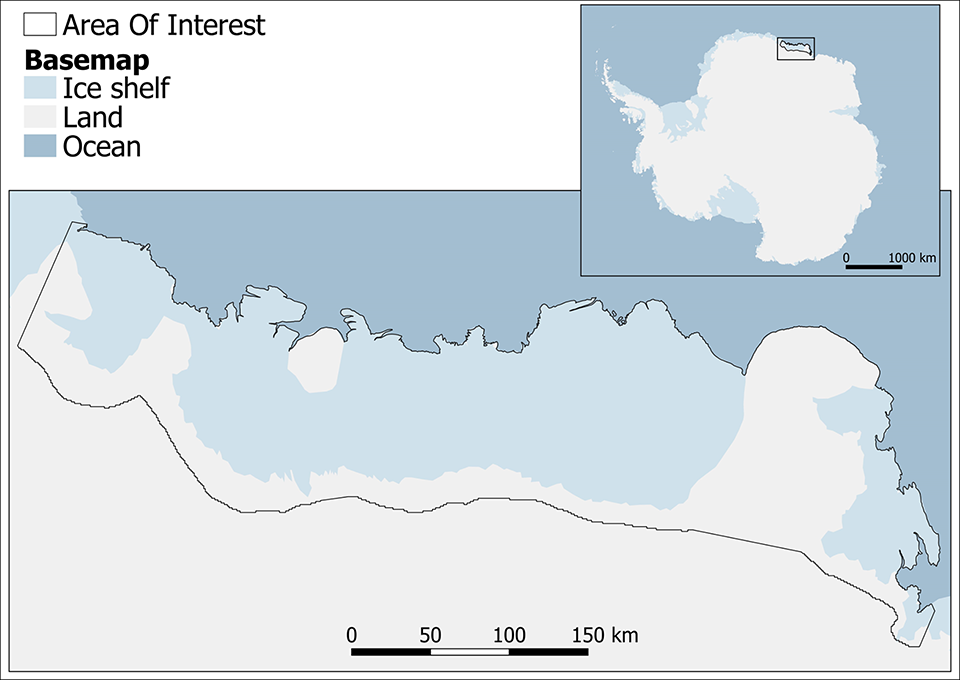
Figure 1. RBIS: the area of interest in East Antarctica. Parts of Prince Harald and Borchgrevink ice shelves are also included in the area as well as the Derwael ice rise and the Riiser-Larsenhalvøya ice ridge (basemap: Quantarctica – Matsuoka et al., 2021, modified)

II. Data presentation

A. MAR Data

7MAR modelling results are gathered in a set of NetCDF files. NetCDF is a common self-document data format used in geosciences for data exchange. It can be seen as a multidimensional datacube. Two of the dimensions are the X and Y coordinates while the third one is time. In our case, each file contains one of the six chosen variables to study. Those variables have similar image size, pixel size, and time resolution (Table 1). The variables are: (i) ME: the melt variable. As SAR has strong interactions with liquid water, this variable would be best correlated with SAR under standardized conditions. As shown in figure 2, ME varies during year, reaching peak value of 10 kg / m² / day. (ii) RO1: the snow density. Divided into the same layers as WA1 (cf. vi), it is not used to be compared directly to SAR data. Together with WA1, it is used to create a variable that represents the relative quantity of water in the snowpack. Typical values of RO1 reach 400-450 kg / m³ on the ice shelf and 600 kg / m³ at the south of the zone. (iii) RU: this variable represents the surface runoff caused by both melt and rainwater. SAR backscatter can change with both, but only the meltwater fraction is studied here. (iv) SMB: the surface mass balance is linked with ablation phenomena and thus may be correlated with the radar cross-section. SMB is calculated as the thickness change of the snowpack. It can be approximated by the sum of all the processes that cause accumulation or ablation. On ice shelves in Antarctica SMB tend to stay quite low and constant with a few kg / km² / day. (v) SU: sublimation is the change from solid-state to gas without passing through the liquid phase. If it is the liquid water that is detected with SAR, for the sublimation process to occur, snow needs heat as it is an endothermic reaction. If there is heat, melting may occur and cause the SAR cross-section to vary. (vi) WA1: WA1 is the liquid water content of snow layers. The file is divided into ten bounds / layers of snow representing the first meter of depth. WA1 can be compared with SAR thanks to the ability of radar frequency to penetrate the soil. During strong melting periods, in the first meter of depth, liquid water content of the snowpack can reach a few percent of the snow mass. A summary of all variables is displayed in table 1.

8For the variables ME and WA1, melt or significant presence of water are considered when the value of the variable is higher than 0.1. This value is then used to create the melting mask used for the quantitative comparison conducted in part III. B.

Variable	Unit	Image size (km)	Pixel size (km)	Time Interval
ME	kg / m² / day	750×720	5 × 5	1 / day
RO1	kg / m³	750 × 720	5 × 5	1 / day
RU	kg / m² / day	750 × 720	5 × 5	1 / day
SMB	kg / m² / day	750 × 720	5 × 5	1 / day
SU	kg / m² / day	750 × 720	5 × 5	1 / day
WA1	kg / kg	750 × 720	5 × 5	1 / day

Table 1. MAR variables used for this study. ME: melt, RO1: snow density, RU: runoff, SMB: surface mass balance, SU: sublimation, WA1: liquid water content

B. SAR Data

9In this study, we used SAR images from the Sentinel-1 mission. It refers to a constellation of two active radar satellites. Sentinel-1 is the first mission of the European Space Agency (ESA) for the Copernicus initiative. Copernicus brings a paradigm shift in the use of remote sensing data. The program aims to provide free, open-access, and high-quality data. The two satellites constituting the constellation (S1A and S1B) work in the C band (5.45 GHz), allowing night and day imagery. With a revisiting time of 12 days, and a near-polar Sun-synchronous orbit, the S1A and S1B allow a revisit time of 6 days. The first satellite – S1A – has been launched in April 2014 for a 7-year mission. In this study, we use data acquired at single and dual polarizations, in interferometric wide (IW) and extra-wide (EW) swaths. For this paper, only the comparison with HH (signal send with a horizontal polarization and received in the same way) polarization is used as the conclusion for the cross polarization HV (signal send horizontally but received vertically) is the same. Over our region of interest, the local period of the descendant node is around 6 PM. The data is retrieved from the Alaska Satellite Facility (ASF, 2021). To preserve the 6 days revisit time of S1A and S1B, the analysis starts in 2016. 1 417 images were used to conduct the analysis. Multiple orbits are used to ensure consistent spatial coverage with MAR data. MAR output temporal resolution can be defined according to the user's needs, but SAR has physical limitations. Even if all the possible data is used, data gaps occur and cause holes in the comparison. Nevertheless, the spatial resolution and pixel size are much finer than MAR. Ground-Range-Detected (GRD) products at high and medium resolution are used for this analysis. These images have a pixel spacing of 10 by 10m and 40 by 40m, respectively.

Pol.	Coeff. (dB)	Acquis.	Pixel size (m)	Time Interval
HH	σ0	IW & EW	10 × 10 & 40 × 40	1 / 6 days
HV	σ0	IW & EW	10 × 10 & 40 × 40	1 / 6 days

Table 2. SAR Data used for this work. Four distinct types of data that are used together, depending on the polarization and acquisition mode

10As explained in the introduction part, the threshold applied for the binary classification used for the quantitative comparison (cf. III. B) is discussed in the literature. The choice is to follow the -2.6 dB threshold proposed by Liang et al. (2021). The co-orbit normalization is not performed as the ice on the iceshelf shows a mean σ0 oscillating around 0 dB.

III. Comparison

11A direct consequence of the different pixel sizes, coverages and data formats between SAR and MAR is the inability to perform a direct comparison without converting the data. For this project, the choice is to downgrade SAR pixel spacing to the 5 km MAR pixel spacing and mosaicking SAR images. A resampling was then included in the SAR processing chain to get images with a 5 by 5 km spatial spacing. The resampling is made with SNAP software (Brockmann et al., 2020), using the default parameters of the Range Doppler Terrain Correction function with the TanDEM-X elevation model data originating from the German aerospace center as used in the frame of the MIMO project (for details see Glaude et al., 2020). The mosaic is created from a Python script. The value of each pixel composing the mosaic for a given date is calculated using linear interpolation (or extrapolation) between the values of two overlaying images. The two chosen images are the couple with the smallest time gab between their acquisition and the given date for the mosaic.

12A mosaic is created every six days to match the six days revisit time of the satellites. The first date of the study is not chosen randomly. It is set in 2016 to benefit from Sentinel A and B and between the acquisition of paths 59 and 88, covering most of the studied zone. The mosaicking of the SAR images is advantageous for different reasons. First the mosaic from multiple SAR images allows us to create maps covering the entire studied region. Such maps offer a synoptic representation of data and underlying phenomena, and they are the basis of spatial analysis. Secondly the use of different paths and orbits can induce variations of σ0 and interpolating a value from multiple images mitigates the variation. Finally, it allows a perfect co-registration of the two datasets by creating a grid over MAR images. This co-registration is ensured by the interpolation of the different layers on the same grid. The upper left corner of MAR and SAR products are coherent, as well as the pixel spacing. The coordinate reference system uses is the Antarctic Polar Stereographic projection (EPSG: 3031).

13However, mosaicking can also lead to artifacts. The major problem is the occurrence of extreme extrapolated values in the case when no data is available in the six days before or after the desired date. A filter is used to reduce the number of extreme values. Furthermore, by interpolating between two images recorded near 6 PM, the intra-daily variations in σ0 are omitted. Dates when the mosaic had an inadequate quality are removed.

14The comparison is made between the satellite data and all the MAR variables previously presented. In the paper, we focus on the results with ME, the variable representing melt, because it is the most consistent with the observation of the satellite.

A. Temporal

15SAR and MAR datasets are first directly compared together. The evolution of the quantity of melt and of σ0 averaged on the ice shelf is displayed in figure 2. A synchronism appears clearly between the decrease of σ0 and the increase in the quantity of melt modelled by MAR. The opposite variation is straightforward since the increase in water concentration in the snowpack leads to a mirror effect in the SAR signal, resulting in a decrease of σ0. However, if the decrease and increase seem to be negatively correlated, it is not the case of the intensity reached by the peaks. The maximum and minimum are not happening for the same melt season and, no matter the quantity of melt modelled by MAR during melt seasons, the same σ0 is observed at –15 / –20 dB. Furthermore, a small temporal shift of one or two weeks between the increase and the decrease is observed. There are two hypotheses to explain that shift. First, MAR tends to model melt too early. Second, a certain quantity of liquid water in the snowpack is required for a change to occur in σ0. Further investigations are needed to test the two hypotheses.

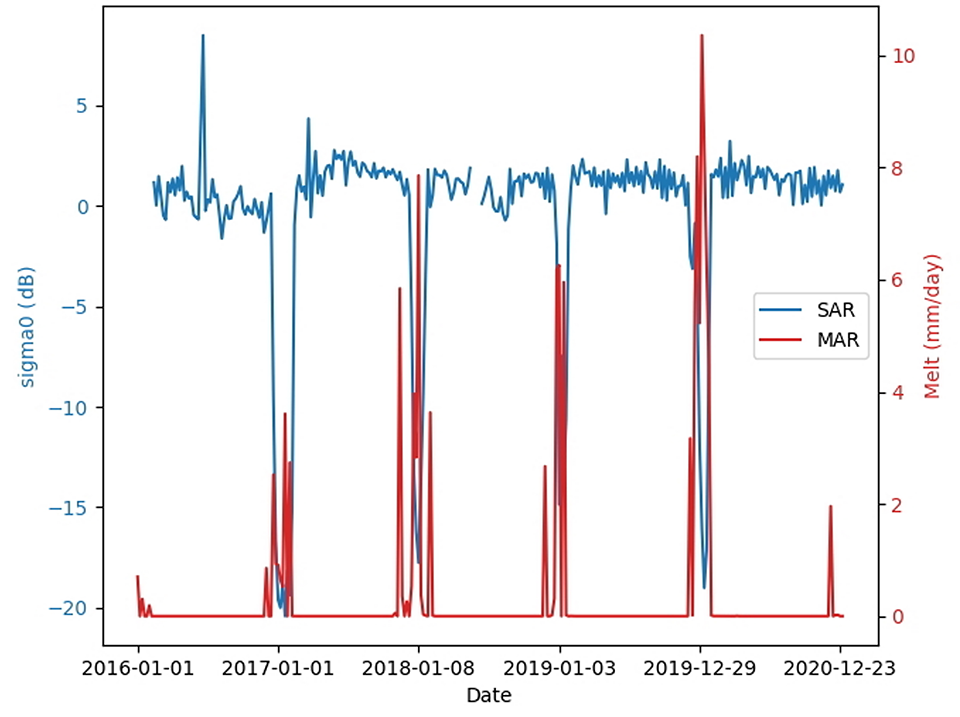
Figure 2. Comparison between SAR σ0 and MAR melt for the studied period of 2016-2021. The opposite variation of the couple of data is explained by the decrease of σ0 caused by the presence of water. Even if the peaks occur at the same time, the increase of ME starts before the decrease of σ₀

16Another temporal comparison is conducted through the construction of two maps: a first one regarding the correlation between σ0 and ME and, a second based on a probability (Equation 1). The correlation map (Figure 3A) uses the value of σ0 observed by the satellite and the ME values given by MAR throughout the whole period studied. With those values, the Pearson’s r is calculated for each pixel, considering every value obtained for the pixel. Roughly 300 couples of ME and σ0 values are used at each pixel for the calculation. The visual interpretation of the result shows strong negative correlation values (~ –0.75) on the ice shelf and lower negative correlation over the slopes and the surrounding ice shelves (~ 0.1). Overall, a gradient appears on the image, with strong correlations near the limit between the ice shelf and the ocean and decreasing toward inland.

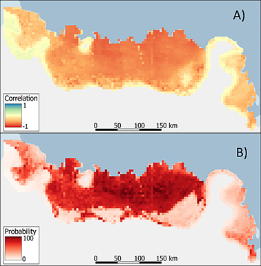
Figure 3. A) Correlation map between SAR σ₀ backscattering coefficient and MAR ME. B) Conditional probability representing the probability of MAR to detect melt, considering SAR observes melt. For both maps, the ice shelves present higher values than over the problematic zones described in part III. B.

17The probability map (Figure 3B) represents the conditional probability of MAR modelling melt given SAR observes it. Following equation 1, this probability is calculated as the ratio between the probability of SAR and MAR both modelling melt and the probability of SAR observing melt. A high probability (~ 90 %) appears on the ice shelf while a low (~ 10 %) probability concerns the blue ice areas, the slopes, and the Prince Harald ice shelf. The low value is due to the SAR over observation of melt in the above-mentioned zones, caused by a threshold choice too high for the zone. On the other hand, the high probability results from the fact that ME is modelled a week or two before and after the observation by SAR.

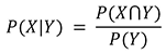
18In equation (1): X states for MAR modelling melt and Y for SAR observing it.

B. Quantitative

19The quantitative analysis is based on the surface melt comparison determined by SAR and by MAR. The comparison is performed on the percentage of the area covered by melt, pixel by pixel, after a binary classification (melt – no melt) of the two variables has been achieved. The melt volume is thus not included in the analysis. Quantifying the melt volume with SAR would deserve more consideration. In figure 4, the time shift is also visible. Melt modelled in the ME variable covers the studied zone before SAR observed a decrease in σ0 and thus before SAR observed an evolution of the surface melt area. The melt modelled area first appears larger than the observed one, before converging to a similar value covering the majority or even the entire studied zone. However, figure 4 also shows the effect of the threshold choice. During the study, a constant melt cover is detected of about 10 to 20 %. There is no period where SAR detects no melt over the studied zone. The cause is to be found in the lack of normalization of the SAR images and the use of a constant threshold instead of a spatially varying one. This resulting melt is mainly located on the slopes – the Prince Harald ice shelf – and the bottom of the slopes, where blue ice is located. When removing these areas from the analysis, the effect is mitigated, and the covered area matches better (Figure 5).

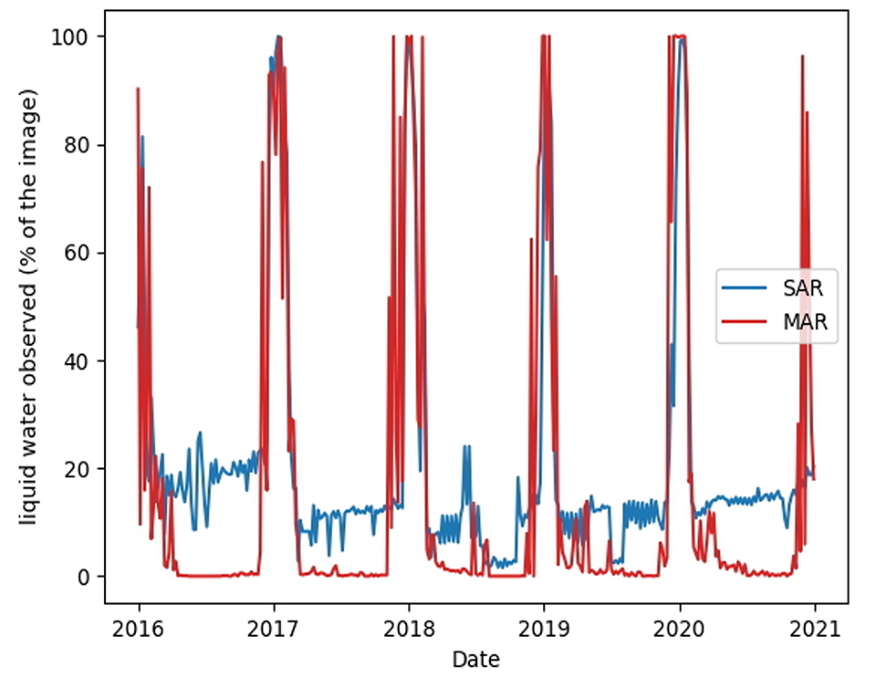
Figure 4. Comparison between SAR and MAR observed liquid water. The comparison is established with the percentage of the area covered by melt. The values for the peaks are equivalent except for the 2021 melt season and the summer period. The difference for 2021 is due to the temporal shift, still visible in the graph. The summer difference is caused by the threshold choice

20Another major difference is the start of the modelled 2021 melt season which covers up to 90 % of the image while it is not observed by SAR. This difference can also be noted in 2016 when the studied zone is restrained.

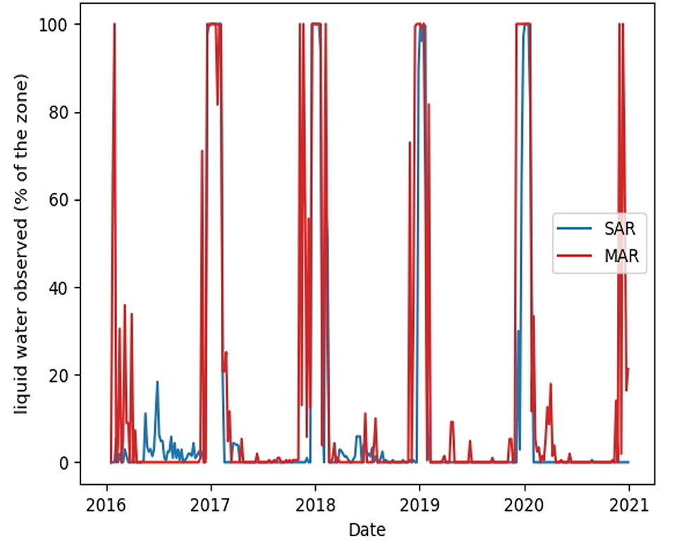
Figure 5. Comparison between SAR and MAR observed liquid water. Graph is identical to figure 4 but the problematic areas have been removed. The differences have decreased but the 2016 melt season has disappeared from SAR

C. Spatial

21The spatial comparison is carried out by analyzing SAR and MAR outputs with the Moran’s I index (Goodchild, 1986). Spatial autocorrelation is the variation of an event with itself in space. An index value of 1 (or -1) reflects a strong positive (or negative) spatial autocorrelation, meaning high values tend to have neighbors with high (or low) values. Neighborhood of a pixels is constructed with a queen-contiguity (8-connexe) at the second order (neighbors of neighbors). The spatial analysis is carried out with the space section of the GeoDa software (Anselin et al., 2006).

22The Moran’s I value (Figure 7A) is significant (0.786) (9999 random permutations test) for the correlation map (Figure 3A). The visual interpretation of the map performed for the temporal analysis is corroborated by the local index analysis (LISA) completed (Figure 6). Values on the slopes are considered as significantly “high-high” (high values surrounded by high values), while the ice shelf is considered as “low-low” (low values surrounded by low values). Topography is then one of the main factors influencing the data variations concerning the correlation as the r coefficient is mainly constant on flat surfaces and tend to vary in areas with strong topographical relief.

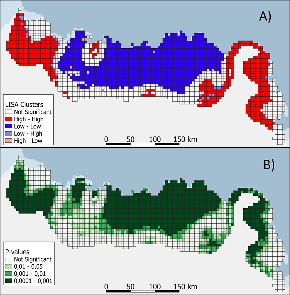
Figure 6. A) Clusters of neighbors, classified according to their LISA index. B) p-value for the LISA indexes, with 9999 permutations. Both maps are constructed for the correlation map.

23For the probability map, Moran’s I (Figure 7B) is also (pseudo-)significant (0.775). However, in this case, the nature of the ice also seems to be significant to explain the differences between the two variables. Nevertheless, it is important to remember that the threshold choice has an impact on the probability as it uses the binary classification of ME and σ0.

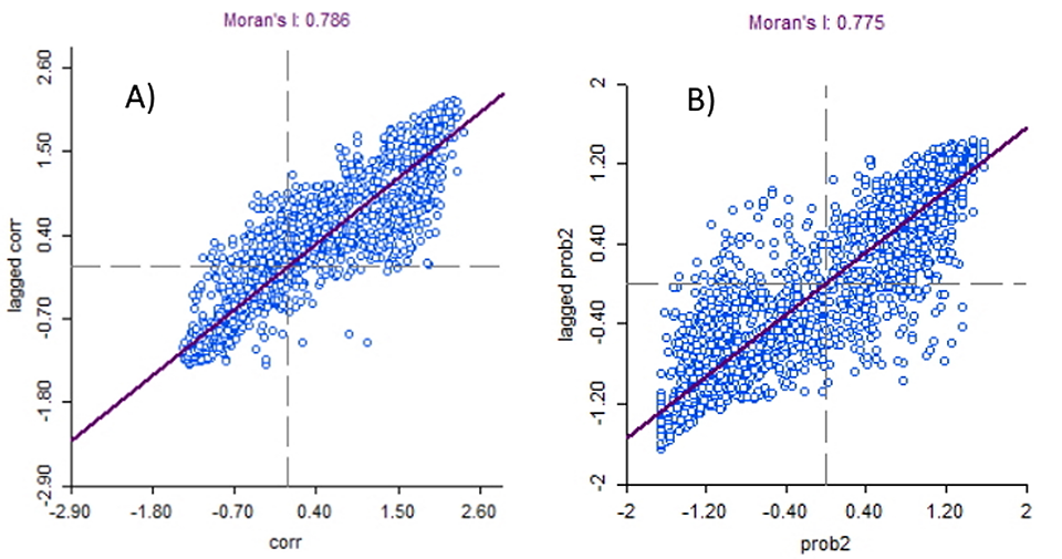
Figure 7. Moran’s I scatterplot for the maps presented at figure 3. The blue dots represent pixels. The X axe is the standardised value of the pixel and Y the mean standardised value of the neighbourhoods. A) Pearson’s r: Moran’s I = 0.786. B) Conditional probability: Moran’s I = 0.775

24So far, the spatial analysis carried out has been limited to the use of simple indicators. More can be done to complete this aspect of the research. First of all, we should explore in more depth the spatial and temporal cross-correlations. Then SAR and MAR data could be investigated by means of a geographically weighted regression in order to analyze the spatial variation of their relationship.

Conclusion and discussion

25In this study, we analyzed the comparison of melt prediction from two independent methods. On the one hand, we are requalifying the backscattering coefficient of SAR remote sensing into a melt / not melt binary classification. On the other hand, we are studying the presence of estimated melt using MAR climate model.

26The results show the complementarity nature of the two datasets. It must be kept in mind that the studied area is firstly modelled by MAR before SAR records it. The temporal shift between ME and σ0 can mainly be caused by the need for a certain quantity of water in the snowpack before observing a variation of σ0. This trend of modelling melt before and after SAR melting observations is also visible in the temporal variation of the melt surface. This consideration aside, the peaks of the melt coverages for the two datasets are consistent with each other (but for the 2021 melt season as it did not start for SAR). The SAR observation of melt during winter is due to the choice of –2.6 dB for the melt threshold. That is too high for some zone that presents lower values in non-melting periods. These zones are highlighted by the spatial analyses carried out with the correlation index and the probability map. Problematic zones have lower probabilities and lower correlation coefficients. However, the results show strong and statistically significant Moran’s I on the ice shelf, blue ice, and the slopes.

27Nevertheless, results could be greatly enhanced by the normalization of SAR images as proposed in Liang et al. (2021) or the use of a spatially variable threshold.

28It would be also possible to conduct the experiment on a larger zone and at a better spatial resolution to benefit from the high resolution of the Sentinel-1 SAR imaging capabilities.

29Finally, MAR and SAR showed similarities for most of the studied zone, and the dissimilarities were observed where the terrain is different, whether because of the nature of the ice or the topography. Further analysis of their differences would benefit the ice sheet modelling field.

References

30Anselin, L., Syabri, I. & Kho, Y. (2006). GeoDa: An introduction to spatial data analysis. Geographical Analysis, 38(1), 5–22. https://doi.org/10.1111/j.0016-7363.2005.00671.x.

31ASF (2021). ASF Data Search. Alaska Satellite facility (ASF). Retrieved 26 May 2021, from https://search.asf.alaska.edu/#/

32Baghdad, N. (2000). Potential and limitations of RADARSAT SAR data for wet snow monitoring. IEEE Transactions on Geoscience and Remote Sensing, 38 (1 I), 316–320. https://doi.org/10.1109/36.823925.

33Berger, S., Favier, L., Drews, R., Derwael, J.J. & Pattyn, F. (2016). The control of an uncharted pinning point on the flow of an Antarctic ice shelf. Journal of Glaciology, 62 (231), 37–45. https://doi.org/10.1017/jog.2016.7.

34Brockmann Consult, Skywatch, Sensar & C-S (2020). SNAP - ESA Sentinel Application Platform v8.0.3 [Computer Software]. Retrieved from http://step.esa.int/.

35Callens, D., Drews, R., Witrant, E., Philippe, M. & Pattyn, F. (2016). Temporally stable surface mass balance asymmetry across an Ice rise derived from radar internal reflection horizons through inverse modeling. Journal of Glaciology, 62 (233), 525–534. https://doi.org/10.1017/jog.2016.41.

36Drews, R. (2015). Evolution of ice-shelf channels in Antarctic ice shelves. Cryosphere, 9 (3), 1169–1181. https://doi.org/10.5194/tc-9-1169-2015.

37Favier, L. & Pattyn, F. (2015). Antarctic ice rise formation, evolution, and stability. Geophysical Research Letters, 42 (11), 4456–4463. https://doi.org/10.1002/2015GL064195.

38Fettweis, X., Gallée, H., Lefebre, F. & van Ypersele, J.P. (2006). The 1988-2003 Greenland ice sheet melt extent using passive microwave satellite data and a regional climate model. Climate Dynamics, 27 (5), 531–541. https://doi.org/10.1007/s00382-006-0150-8.

39Fettweis, X., Tedesco, M., Van Den Broeke, M. & Ettema, J. (2011). Melting trends over the Greenland ice sheet (1958-2009) from spaceborne microwave data and regional climate models. Cryosphere, 5 (2), 359–375. https://doi.org/10.5194/tc-5-359-2011.

40Gilbert, E. & Kittel, C. (2021). Surface Melt and Runoff on Antarctic Ice Shelves at 1.5°C, 2°C, and 4°C of Future Warming. Geophysical Research Letters, 48 (8), 1–9. https://doi.org/10.1029/2020GL091733.

41Glaude, Q., Amory, C., Berger, S., Derauw, D., Pattyn, F., Barbier, C. & Orban, A. (2020). Empirical Removal of Tides and Inverse Barometer Effect on DInSAR from Double DInSAR and a Regional Climate Model. IEEE Journal of Selected Topics in Applied Earth Observations and Remote Sensing, 13, 4085–4094. https://doi.org/10.1109/JSTARS.2020.3008497.

42Goldberg, D., Holland, D.M. & Schoof, C. (2009). Grounding line movement and ice shelf buttressing in marine ice sheets. Journal of Geophysical Research: Earth Surface, 114 (4), 1–23. https://doi.org/10.1029/2008JF001227.

43Goodchild, M.F. (1986). Spatial Autocorrelation. Concepts and Techniques in Modern Geography (CATMOG), 47. Norwich : Geobooks, 57 p.

44IMBIE team (2018). Mass balance of the Antarctic Ice Sheet from 1992 to 2017. Nature, 558, 219–222. https://doi.org/https://doi.org/10.1038/s41586-018-0179-y.

45Johnson, A., Fahnestock, M. & Hock, R. (2020). Evaluation of passive microwave melt detection methods on Antarctic Peninsula ice shelves using time series of Sentinel-1 SAR. Remote Sensing of Environment, 250 (2020), 9p. https://doi.org/10.1016/j.rse.2020.112044.

46Koskinen, J.T., Pulliainen, J.T. & Hallikainen, M.T. (1997). The use of ERS-1 SAR data in snow melt monitoring. IEEE Transactions on Geoscience and Remote Sensing, 35 (3), 601–610. https://doi.org/10.1109/36.581975.

47Liang, D., Guo, H., Zhang, L., Cheng, Y., Zhu, Q. & Liu, X. (2021). Time-series snowmelt detection over the Antarctic using Sentinel-1 SAR images on Google Earth Engine. Remote Sensing of Environment, 256, 112318. https://doi.org/10.1016/j.rse.2021.112318.

48Lievens, H., Demuzere, M., Marshall, H.P., Reichle, R.H., Brucker, L., Brangers, I., de Rosnay, P., Dumont, M., Girotto, M., Immerzeel, W.W., Jonas, T., Kim, E.J., Koch, I., Marty, C., Saloranta, T., Schöber, J. & De Lannoy, G.J.M. (2019). Snow depth variability in the Northern Hemisphere mountains observed from space. Nature Communications, 10 (1), 1–12. https://doi.org/10.1038/s41467-019-12566-y.

49Matsuoka, K., Skoglund, A., Roth, G., de Pomereu, J., Griffiths, H., Headland, R., Herried, B., Katsumata, K., Le Brocq, A., Licht, K., Morgan, F., Neff, P.D., Ritz, C., Scheinert, M., Tamura, T., Van de Putte, A., van den Broeke, M., von Deschwanden, A., Deschamps-Berger, C. & Melvær, Y. (2021). Quantarctica, an integrated mapping environment for Antarctica, the Southern Ocean, and sub-Antarctic islands. Environmental Modelling and Software, 140. https://doi.org/10.1016/j.envsoft.2021.105015.

50Moreira, A., Prats-iraola, P., Younis, M., Krieger, G., Hajnsek, I. & Papathanassiou, K.P. (2013). SAR-Tutorial-March-2013. IEEE Geoscience and Remote Sensing Magazine, 1 (1), 6–43. https://doi.org/10.1109/MGRS.2013.2248301.

51Nagler, T. & Rott, H. (2000). Retrieval of wet snow by means of multitemporal SAR data. IEEE Transactions on Geoscience and Remote Sensing, 38 (2 I), 754–765. https://doi.org/10.1109/36.842004.

52Nagler, T., Rott, H., Hetzenecker, M., Wuite, J. & Potin, P. (2015). The Sentinel-1 mission: New opportunities for ice sheet observations. Remote Sensing, 7 (7), 9371–9389. https://doi.org/10.3390/rs70709371.

53Nagler, T., Rott, H., Ripper, E., Bippus, G. & Hetzenecker, M. (2016). Advancements for snowmelt monitoring by means of Sentinel-1 SAR. Remote Sensing, 8 (4), 1–17. https://doi.org/10.3390/rs8040348.

54Navari, M., Margulis, S.A., Bateni, S.M., Tedesco, M., Alexander, P. & Fettweis, X. (2016). Feasibility of improving a priori regional climate model estimates of Greenland ice sheet surface mass loss through assimilation of measured ice surface temperatures. Cryosphere, 10 (1), 103–120. https://doi.org/10.5194/tc-10-103-2016.

55Navari, M., Margulis, S.A., Tedesco, M., Fettweis, X. & Alexander, P.M. (2018). Improving Greenland Surface Mass Balance Estimates Through the Assimilation of MODIS Albedo: A Case Study Along the K-Transect. Geophysical Research Letters, 45 (13), 6549–6556. https://doi.org/10.1029/2018GL078448.

56Paolo, F.S., Fricker, H.A. & Padman, L. (2015). Volume loss from Antarctic ice shelves is accelerating. Science, 348 (6232), 327–331. https://doi.org/10.1126/science.aaa0940.

57Pattyn, F. (2018). The paradigm shift in Antarctic ice sheet modelling. Nature Communications, 9 (1), 10–12. https://doi.org/10.1038/s41467-018-05003-z.

58Payne, A.J., Vieli, A., Shepherd, A.P., Wingham, D.J. & Rignot, E. (2004). Recent dramatic thinning of largest West Antarctic ice stream triggered by oceans. Geophysical Research Letters, 31 (23), 1–4. https://doi.org/10.1029/2004GL021284.

59Pollard, D., DeConto, R.M. & Alley, R.B. (2015). Potential Antarctic Ice Sheet retreat driven by hydrofracturing and ice cliff failure. Earth and Planetary Science Letters, 412, 112–121. https://doi.org/10.1016/j.epsl.2014.12.035.

60Pritchard, H.D., Arthern, R.J., Vaughan, D.G. & Edwards, L.A. (2009). Extensive dynamic thinning on the margins of the Greenland and Antarctic ice sheets. Nature, 461 (7266), 971–975. https://doi.org/10.1038/nature08471.

61Pritchard, H.D., Ligtenberg, S.R.M., Fricker, H.A., Vaughan, D.G., Van Den Broeke, M.R. & Padman, L. (2012). Antarctic ice-sheet loss driven by basal melting of ice shelves. Nature, 484 (7395),502–505. https://doi.org/10.1038/nature10968.

62Scambos, T., Hulbe, C. & Fahnestock, M. (2013). Climate-Induced Ice Shelf Disintegration in the Antarctic Peninsula. Antarctic Peninsula Climate Variability, 79, 79–92. https://doi.org/10.1029/ar079p0079.

63Shah, E., Jayaprasad, P. & James, M.E. (2019). Image Fusion of SAR and Optical Images for Identifying Antarctic Ice Features. Journal of the Indian Society of Remote Sensing, 47 (12), 2113–2127. https://doi.org/10.1007/s12524-019-01040-3.

64Wingham, D.J., Shepherd, A., Muir, A. & Marshall, G.J. (2006). Mass balance of the Antarctic ice sheet. Philosophical Transactions of the Royal Society A: Mathematical, Physical and Engineering Sciences, 364 (1844), 1627–1635. https://doi.org/10.1098/rsta.2006.1792.

Para citar este artículo

Acerca de: Thomas DETHINNE

Acerca de: Quentin GLAUDE

Acerca de: Charles AMORY

Acerca de: Christoph KITTEL

Acerca de: Xavier FETTWEIS