


- Portada
- volume 10 (2006)
- numéro 3
- Design of a micro-irrigation system based on the control volume method


Vista(s): 5047 (16 ULiège)
Descargar(s): 0 (0 ULiège)

Design of a micro-irrigation system based on the control volume method

Notes de la rédaction
Received 5 April 2005, accepted 24 January 2006
Résumé
Dimensionnement de système de micro-irrigation basé sur la méthode du volume de contrôle. Le dimensionnement du système de micro-irrigation basé sur la méthode du contrôle de volume et utilisant la procédure « back step » est présenté dans cette étude. La méthode numérique proposée est simple et consiste à isoler un volume élémentaire de la rampe, muni d’un goutteur et de longueur égale à l’espacement entre deux goutteurs. A ce volume de contrôle, sont appliquées les équations fondamentales de conservation relatives à l’hydrodynamique du fluide. La méthode de contrôle de volume repose sur un principe de calcul itératif de la vitesse et de la pression, pas à pas, pour l’ensemble du réseau. A l’aide d’un simple programme informatique, les équations établies sont résolues et la convergence vers la solution est rapide. Connaissant les besoins en eau d’une culture, il est cependant aisé de choisir sur la base d’un débit moyen des goutteurs, le débit global du réseau. Ce calcul permet de repérer les dimensions économiques des conduites du réseau, assurant une uniformité de distribution d’eau acceptable (95 %). Ce programme permet de dimensionner des réseaux complexes ayant des milliers de goutteurs et offre la possibilité de choisir le réseau optimal. Il donne la vitesse et la pression en n’importe quel point du réseau. Ce programme relativement simple a été testé pour le dimensionnement de la rampe et les résultants sont similaires à ceux obtenus par la méthode des éléments finis.
Abstract
A micro-irrigation system design based on control volume method using the back step procedure is presented in this study. The proposed numerical method is simple and consists of delimiting an elementary volume of the lateral equipped with an emitter, called « control volume » on which the conservation equations of the fluid hydrodynamic’s are applied. Control volume method is an iterative method to calculate velocity and pressure step by step throughout the micro-irrigation network based on an assumed pressure at the end of the line. A simple microcomputer program was used for the calculation and the convergence was very fast. When the average water requirement of plants was estimated, it is easy to choose the sum of the average emitter discharge as the total average flow rate of the network. The design consists of exploring an economical and efficient network to deliver uniformly the input flow rate for all emitters. This program permitted the design of a large complex network of thousands of emitters very quickly. Three subroutine programs calculate velocity and pressure at a lateral pipe and submain pipe. The control volume method has already been tested for lateral design, the results from which were validated by other methods as finite element method, so it permits to determine the optimal design for such micro-irrigation network.
Tabla de contenidos
1. Introduction
1The finite element method (FEM) is a systematic numerical procedure that has been used to analyse the hydraulics of the lateral pipe network. A finite element computer model was developed by Bralts and Segerlind (1985) to analyse micro-irrigation submain units. The advantage of their technique included minimal computer storage and application to a large micro-irrigation network. Bralts and Edwards (1986) used a graphical technique for field evaluation of micro-irrigation submain units and compared the results with calculated data. Micro-irrigation system design was analysed using the microcomputer program by Bralts et al. (1991). This program provided the pressure head and flows at each emitter in the system. The program also gave several useful statistics and provided an evaluation of hydraulic design based upon simple statistics and economics criteria. Since the number of laterals in such a system is large, Bralts et al. (1993) proposed a technique for incorporating a virtual node structure, combining multiple emitters and lateral lines into virtual nodes. After developing these nodal equations, the FEM was used to numerically solve nodal pressure heads at all emitters. This simplification of the node number reduced the number of equations and was easy to calculate with a personal computer.
2Most numerical methods for analysing micro-irrigation systems utilise the back step procedure, an iterative technique to solve for flow rates and pressure heads in a lateral line based on an assumed pressure at the end of the line. However, a micro-irrigation network program needs « large » computer memory, and a long computer calculation time due to the large matrix equations.
3A mathematical model was also developed for a microcomputer by Hills and Povoa (1993) analysing hydraulic characteristics in a micro-irrigation system including emitter plugging. An iterative procedure was used to locate the average pressure using the Newton-Secant Method. Kang and Nishiyama (1994) and Kang and Nishiyama (1996a) used the finite element method to analyse the pressure head and discharge distribution along the lateral lines and submains. A golden section search was applied (Kang, Nishiyama, 1996 b) to find the operating pressure heads of the lateral and submain lines corresponding to the required uniformity of water application. A computer program was developed using the back step procedure.
4The primary objective of the present study is to develop and implement a simple program for the hydraulic analysis of lateral pipes and the micro-irrigation system. Using the back step procedure and control volume method (CVM), results in a non-linear system of algebraic equations, where pressure and velocity are coupled. The objective is to simultaneously solve these equations. The use of the control volume method reduced computing time required in FEM and facilitated computations.
5The principal computation program was developed in Fortran language using three subroutine control volume programs; a lateral pipe program and a submain program. This computation program analysed the head pressure and discharge distribution along the lateral and submain pipes and gave total flow rate and total operating pressure of network.
2. Theoretical development
6The proposed computation model was based upon equations of conservation of mass and energy applied to an elementary control volume, containing one emitter on one lateral or submain pipe and solved by the use of the back step procedure. The first control volume is chosen at the end of the last lateral pipe of network to find pressure at the entrance to the lateral pipe HLmax, or pressure at the end of lateral pipe HLmin. The iterative process based on the back step procedure was successively applied until the other lateral extremity and for all the network (Figure 1). The calculation was continued step-by-step using an iteration process for all the submain units.
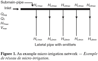
7Figure 1 shows the total average flow rate of network Qavg in m3.s-1, which is an input for the computation, the total flow rate QT in m3.s-1 given after computation, the total head pressure HTmax in m and the velocity Vmax in m.s-1 at network entrance.
8The total network is formed by the identical laterals presented in figure 2.
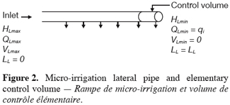
9In figure 2, HLmax represents the pressure at lateral entrance, Qmax represents the total flow rate at lateral pipe entrance, Vmax the velocity at lateral pipe entrance, HLmin the pressure at the end of lateral pipe (LL = LL), VLmin the velocity at the end of lateral pipe, Q = qi the discharge of last emitter and LL the length of lateral pipe.
10For the elementary volume (Figure 3), the principles of mass and energy conservation are applied.
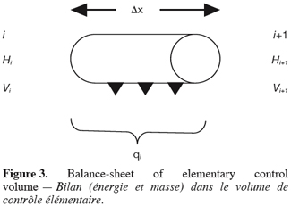
11The ith emitter discharge qi in m3.s-1 is assumed to be uniformly distributed along the length between emitters ∆xL, and is given by:

12(1)
13or

14(2)
15where a is an empirical constant; y is the emitter exponent; Hi, Hi+1 respectivelly the pressure at ith and (i+1)th point. H is the average pressure along DxL. The mass conservation equation for the control volume gives:
16Mi/t = Mi+1/t + qi
17(3)
18where Mi in kg is water mass at the entrance of the control volume, Mi+1 in kg water mass at the exit control volume and t time in s, (M=rW; r is volumic mass of water, W is volume).
19The energy conservation between i and i+1 is as follows:
20Ei = Ei+1 + DH
21(4)
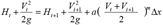
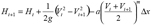
22where Ei is flow energy or pressure in at the input and Ei+1 is flow energy at the exit; and DH including the local head loss hf due to the emitter is the head loss in m due to friction along DxL. The head losses DH are given by the following formula:

23(5)
24or
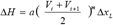
25(6)
26VL in m.s-1, is the avarage velocity between i and (i+1), Vi and Vi+1 are velocity respectively at ith and (i+1)th cross-section lateral, the value of parameter a is given by Hazen-William equations:
27for turbulent flow, Re is Reynold’s number, Re > 2300,

28(7)
29for laminar flow, Re < 2300,

30(8)
31where C is Hazen-William coefficient; K proportion-able coefficient; m exponent (m = 1 for laminar flow, m = 1.852 for turbulent flow); AL cross-sectional area of lateral pipe in m2; DL interior lateral pipe diameter in m; n kinematic viscosity in m2.s-1; g gravitational acceleration in m.s-2. HL and VL are respectively the average pressure and the average velocity between ith and (i+1)th emitter on the lateral. The calculation model for lateral pipe solves simultaneously the system of two coupled and non-linear algebraic equations, having two unknown values:
32Vi+1 and Hi+1.
33Equations (3) and (4) become:
34ALVi = ALVi+1 + qi
35(9)
36(10)
37and equations (9) and (10) become:

38(11)
39(12)
40For the lateral, equations (11) and (12) become:

41(13)

42(14)
43For submain pipe, equations system is

44(15)

45(16)
46where Qs is flow rate in submain pipe, As a cross-sectional area of submain pipe, Vs and Hs respectively, velocity and pressure in submain pipe. At the end of the lateral Vi = 0, HLmax is given at entrance of lateral pipe, inlet head pressure. The slop of lateral and submain pipe are assumed null (plat level).
47When HLmax is fixed, the computation program of lateral can give the distribution velocity or emitter’s discharge and pressure along lateral. Theoretical development giving equations (11), (12) and (13), (14) was already solved without the use of matrix algebra through CVM or Runge Kutta presented in another paper (Zella et al., 2003 ) and (Zella, Kettab, 2002).
2.1. Iterative procedure
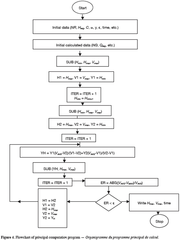
48The numerical calculation is accomplished using calculation program in Fortran 77 for the micro-computer. The details of the program are included in the flowchart in figure 4.
49Step 1: to fix HLmin, VLmin = 0
50HLmin, VLmin are respectively the pressure and the velocity at the end of lateral.
51Step 2: to calculate equations system (11) and (12) or (13) and (14), so QL = Qs corresponding to HLmin and HLmax will be known.
52Step 3: to calculate Vs using equation (15) and Hs using equation (16)
53Using linear approximation, the convergence to solution is given by: HLmax, Hsmax and Vsmax. The test of convergence is based on the two equations (17) and (18) with e the precision of imposed to the solution:

54(17)

55(18)
2.2. Uniformity calculation
56The discharge of any emitter on lateral is given by typical relation equation (1), the average discharge of emitter qavg is considered for all discharge emitters on lateral (NG), total discharge QL or Qmax at lateral entrance and the total average discharge QL avg corresponding to average pressure HL avg are evaluated respectively by the following equations where qn is the nominal emitter discharge.
57Qmax = VLmax A
58(19)
59QLavg = NG.qn
60(20)

61(21)

62(22)
63The coefficients variation for discharge or pressure are the quotient between standard deviation and values of average emitter discharge or average pressure:

64(23)

65(24)
66The coefficient of discharge uniformity (Cuq) and pressure uniformity (CuH) are calculated by the following (Bralts et al., 1993) equations:
67Cuq = 100(1-Cvq)
68(25)
69CuH = 100(1-CvH)
70(26)
3. Applications and Results
3.1. Lateral design examples
71A horizontal lateral pipe (slope = 0%) of length LL = 250 m and the interior diameter DL = 15.2 mm. The Hazen-William coefficients of polyethylene tubing are C = 150, m = 1.852 and K = 5.88 and the water kinematic viscosity is n = 10-6 m2.s-1. The emitter spacing DxL is equal to 5 m, so the number of emitter per lateral is NG = 50. The emitter constant and exponent are, respectively a = 9.14.10-7, and y = 0.5. The required precision for the test of convergence is e = 10-6.
72The computation program using the CVM provided the distribution of discharge and pressure with different values of head pressure, HLmax (Table 1). The uniformity coefficient increased with HLmax while all other parameters (diameter, length, emitter, spacing) were constant. As pressure increased from 20 to 60 m or 75% of the highest HLmax, the new uniformity coefficient, Cuq increased only by 0.56%. This shows that it is useless to opt for the elevated HLmax values since the uniformity of distribution doesn’t improve. If the increase of Cuq is required, it is necessary to change diameter of lateral line or the type of emitters. The elevated value of Hmax is a waste of pumping energy. Water uniformity (≈ 95%) guaranteed to satisfy water needs of plants when variation of pressure and emitter discharge were, respectively, less than 20% and 10%.
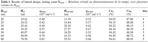
73The example illustrated in figure 5 is a result obtained by the computation program based on the CVM, the curve permits to know the pressure along the lateral line and therefore at each emitter. This results is the same as one obtained by Bralts et al. (1993) using the finite element method. The convergence is reached after 8 iterations and a computer time of 4 seconds compared to 3 iterations and one second for FEM and CVM, respectively. The CVM model can be considered validated by reaching the same result as the FEM model of Bralts et al. (1993) which was validated by the « exact » method.
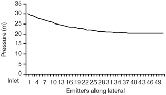
3.2. Network design examples
74Case 1: Simple unit submain as shown in figure 1. A horizontal submain pipe was considered (slope = 0%) with a length Ls = 50 m, a diameter Ds = 0.025 m, and a lateral number NR = 10. All the laterals are identical and their characteristics have been defined in the previous example (LL = 250 m, DL = 1.52.10-2 m). The emitters are also the same, so the total number of emitters is NGT = 500 and the calculation precision is maintained equal to e = 10-3.
75After the network program computation, the total pressure was found HTmax = 44.23 m, the maximal velocity Vmax = 4.80 m/s, and the flow rate QT = 2.357 l/s.
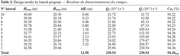
76These results of the network program were verified by the execution of the lateral program for the 10 laterals network. For the 10th lateral, fixed to the extremity of submain pipe, the total flow rate was QL = 0.2172.10-3 l.s-1 for input pressure HLmax = 30 m, Figure 5 represents the distribution of the pressure along lateral pipe. Between the 10th and the 9th lateral, the pressure loss was determined by the Darcy-Weisbach equation as DHs = 0.062 m. The calculation is achieved for the ten laterals and results are regrouped in table 2. The difference between the average flow rate Qavg project and the total flow rate, QT, given after computation was only 3.9.10-3 l/s. It means Qavg introduced by designer data was completely distributed for all emitters.
77Water and mineral elements are delivered to a localised place, to the level of each plant by the emitters whose discharge is function of lateral pressure. The precision of irrigation application, which must exactly satisfy the requirement for cultivation, depends fundamentally on the design of the network. It takes into account the pressure variations, which are due not only to head loss in the pipes of network but also to the land slope, characteristics of emitter, water and air temperature and the possible plugging of emitter orifice.
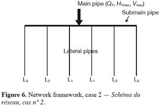
78Case 2: Inlet flow rate at middle of submain. The network (Figure 6) was composed with 2 symmetric submain pipes with the same data as case 1. HTmax = 36.147 m, Vmax = 2.40 m/s, QT = 2.356 l/s.
79The network program is tested for this case of micro-irrigation network. Results were correct and precise at entrance of the submain pipe. The average flow rate, Qavg, was distributed completely between emitters, assuring zero velocity to the extremity of every lateral pipe and a superior distribution uniformity to 94.22%. The difference between the average flow rate of project Qavg and QT, given after computation is only 3.9.10-3 l.s-1. Results are essentially instantaneously given and the computer time was very short.
80Case 3: A network as described in Figure 1 with the same data. The results after computation are shown for several NR (Ls = 50 m) in table 3.
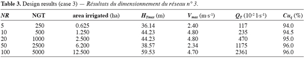
81For NR = 50 and NR = 100, submain diameter is 0.08 m, because with Ds = 0.025 m there is no solution, the flow rate is high exciting a very important head losses in submain and laterals. In these cases, velocities are very high and it’s necessarily to increase more submain diameter in order to obtain value around 1.5 m.s-1.
82These results show that the computer program operates well and converges quickly toward fixed (Qavg) solution at the desired uniformity. The uniformity of emitters distribution is superior to 94.22% for these tested cases. The program gave some precise results for networks covering an irrigated area of 12.5 ha totalling 5000 emitters. In order to analyse such a large micro-irrigation system accurately and efficiently, the task of calculating the pressure and discharges for each emitter becomes enormous so it’s important to choose this computation method.
4. Conclusion
83The control volume method was tested and validated for the lateral design and was used in this paper for designing a simple micro-irrigation network. The model precisely describes the distribution of pressure and discharges to all network emitters. In this case, the total discharge and the total required pressure, the uniformity of pressure and discharges are determined for each pattern of design. The combination of size network pipes and uniformity distribution (plants water requirement) is applied to guarantee an optimal exploitation taking into account the limits imposed by the specific norms for micro-irrigation and the technical limits of velocity and pressure tolerance. Uniformity of water distribution is a main criterion for network design. A microcomputer program was developed that permits designs of high precision in order to optimise the water distribution uniformity at a reasonable investment cost. The proposed methodology is computationally efficient and can help irrigation consultants in the design of micro-irrigation system. In arid and semiarid regions, design is important to increase yields and to conserve water and soil as well as the economical utilisation of power.
84Notations
85a: empirical constant of emitter
86n: kinematic viscosity of water (m2.s-1)
87e: precision of convergence (%)
88s: standard deviation of average discharge emitter (%)
89DH: head loss along the length of control volume Dx (m)
90DHL: head loss along the length lateral pipe (LL) (m)
91DHS: head loss along the length submain pipe (Ls) (m)
92DxL: spacing between emitters (m)
93DxS : spacing between laterals (m)
94a: coefficient of head loss (Hazen-William)
95AL: cross-sectional area lateral pipe, m2
96As: cross-sectional area submain pipe, m2
97C: Hazen-William coefficient
98CuH: coefficient of pressure uniformity at the lateral pipe (%)
99Cuq: coefficient of discharge uniformity at the lateral pipe (%)
100CvH: coefficient of variation of pressure emitter (%)
101Cvq: coefficient of variation of discharge emitter (%)
102DL: interior lateral pipe diameter (m)
103Ds: interior diameter of submain pipe (m)
104Ei: water energy at entrance of control volume (m)
105Ei+1: water energy at exit of control volume (m)
106g: gravitational acceleration (m.s-2)
107HL1: pressure of emitter number 1 at the lateral (≈ HLmax) (m)
108HL50: pressure of emitter number 50 at the lateral (= HLmin) (m)
109HLavg: average pressure at lateral in m corresponding to average discharge QLavg (m3.s-1)
110HLmax: pressure at the entrance to the lateral pipe (m)
111HLmin: pressure at the end of the lateral pipe (m)
112Hs: pressure in submain pipe (m)
113Hsmax: pressure at the entrance submain pipe (m)
114HTmax: the total pressure of the network (m)
115Iter: number of computation iteration
116K: coefficient of proportionality
117LL: the length of the lateral pipe (m)
118Ls: length of submain pipe, m
119m: exponent of regime flow
120Mi: water mass at the entrance of control volume (kg)
121Mi+1: water mass at exit of control volume (kg)
122NG: number of emitters on lateral
123NGT: total number of emitter of network
124NR: number of lateral pipe of network
125qavg: average discharge of emitters (m3.s-1)
126Qavg: the total average flow rate of the network, input data (m3.s-1)
127qi: the discharge of emitter i (m3.s-1)
128Qmax (= QL): the total flow rate at the lateral entrance (m3.s-1)
129qn: nominal discharge of emitter (m3.s-1)
130Qs: flow rate in submain (m3.s-1)
131QT: the total average flow rate of the network given by computation, output data (m3.s-1)
132Re: Reynolds number
133t: time (s)
134VLmax: the velocity at the lateral pipe entrance (m.s-1)
135VLmin: the velocity at the end of the lateral pipe (m.s-1)
136Vmax: the velocity at the network entrance (m.s-1)
137Vs: velocity in submain (m.s-1)
138Vsmax: velocity at the entrance submain pipe (m.s-1)
139y: emitter exponent
Bibliographie
Bralts VF., Segerlind LJ. (1985). Finite element analysis of drip irrigation submain units. Trans. Am. Soc. Agric. Eng. 28 (3), p. 809–814.
Bralts VF., Edwards DM. (1986). Field evaluation of submain units. Trans. Am. Soc. Agric. Eng. 29 (6), p. 1659–1664.
Bralts VF., Shayya WH., Driscoll MA., Cao L. (1991). An expert system for the hydraulic design of microirrigation systems. International Summer Meeting, ASAE, New Mexico, paper n° 91-2153, 12 p.
Bralts VF., Kelly SF., Shayya WH., Segerlind LJ. (1993). Finite element analysis of microirrigation hydraulics using a virtual emitter system. Trans. Am. Soc. Agric. Eng. 36 (3), p. 717–725.
Hills DJ., Povoa AF. (1993). Pressure sensivity to microirrigation emitter plugging. International Summer Meeting, ASAE/CSAE, Washington. Paper n° 93-2130, 17 p.
Kang Y., Nishiyama S. (1994). Finite element method analysis of microirrigation system pressure distribution. Trans. Jap. Soc. Irrig. Drain. Reclam. Eng. 169, p. 19–26.
Kang Y., Nishiyama S. (1996 a). Analysis and design of microirrigation laterals. J. Irrig. Drain. Eng. 122 (2), march/april, ASCE, p. 75–82.
Kang Y., Nishiyama S. (1996 b). Design of microirrigation submain units. J. Irrig. Drain. Eng. 122 (2), march/april, ASCE. p. 83–90.
Zella L., Kettab A. (2002). Numerical methods of microirrigation lateral design. Biotechnol. Agron. Soc. Environ. 6 (4), p. 231–235.
Zella L., Kettab A., Chasseriaux G. (2003). Hydraulic simulation of micro-irrigation lateral using control volume method. Agronomie 23 (1), p. 37–44.
