Angélique Delafosse, Frank Delvigne, Marie-Laure Collignon, Michel Crine, Philippe Thonart & Dominique Toye

Development of a compartment model based on CFD simulations for description of mixing in bioreactors

Document(s) associé(s)

Annexes

• version pdf

Résumé

Développement d'un modèle compartimenté basé sur la mécanique des fluides numérique pour la description du mélange en bioréacteur. La compréhension et la modélisation des interactions complexes entre l'hydrodynamique et les réactions biologiques sont un véritable challenge dans les bioprocédés. Il est nécessaire de proposer des outils numériques capables de rendre compte de ces interactions. La simulation numérique (CFD) permet de décrire en détail l'écoulement au sein d'un réacteur mais elle reste encore aujourd'hui peu réalisable lorsque l'on veut modéliser des réactions complexes. Une autre possibilité est l'utilisation de modèles compartimentés beaucoup moins couteux en temps de calcul. Cependant, ce type de modèle est souvent basé sur des grandeurs globales peu représentatives de la complexité de l'écoulement au sein d'un bioréacteur. Une troisième solution est de coupler les deux précédentes méthodes en définissant un modèle compartimenté basé sur une simulation CFD. La difficulté de ce modèle hybride réside dans la définition des compartiments du modèle de manière à ce qu'ils puissent être considérés comme homogènes. La définition des compartiments peut se faire de manière « manuelle » ou automatique. Dans ce travail, ces deux manières de compartimenter un bioréacteur ont été utilisées et comparées en suivant le mélange d'un traceur inerte. Plusieurs critères pour la définition des compartiments ainsi que plusieurs algorithmes permettant l'automatisation ont été développés dans ce travail.

Abstract

Understanding and modeling the complex interactions between biological reaction and hydrodynamics are a key problem when dealing with bioprocesses. It is fundamental to be able to accurately predict the hydrodynamics behavior of bioreactors of different size and its interaction with the biological reaction. CFD can provide detailed modeling about hydrodynamics and mixing. However, it is computationally intensive, especially when reactions are taken into account. Another way to predict hydrodynamics is the use of "Compartment" or "Multi-zone" models which are much less demanding in computation time than CFD. However, compartments and fluxes between them are often defined by considering global quantities not representative of the flow. To overcome the limitations of these two methods, a solution is to combine compartment modeling and CFD simulations. Therefore, the aim of this study is to develop a methodology in order to propose a compartment model based on CFD simulations of a bioreactor. The flow rate between two compartments can be easily computed from the velocity fields obtained by CFD. The difficulty lies in the definition of the zones in such a way they can be considered as perfectly mixed. The creation of the model compartments from CFD cells can be achieved manually or automatically. The manual zoning consists in aggregating CFD cells according to the user's wish. The automatic zoning defines compartments as regions within which the value of one or several properties are uniform with respect to a given tolerance. Both manual and automatic zoning methods have been developed and compared by simulating the mixing of an inert scalar. For the automatic zoning, several algorithms and different flow properties have been tested as criteria for the compartment creation.

Table des matières

1. Introduction

1Understanding and modeling the complex interactions between biological reaction and hydrodynamics are a key problem when dealing with bioprocesses. The scale-up of a bioprocess from lab-scale to industrial scale often results in a decrease of the productivity compared to the lab-scale one (Enfors et al., 2001). This problem can be partly attributed to the decreasing mixing efficiency with the increasing bioreactor size. Indeed, strong gradients (substrate, dissolved oxygen, pH, etc.) appear when the bioreactor volume increases and can lead to modifications of the biological responses in terms of physiology or/and metabolism compared to lab-scale cultures (Enfors et al., 2001). It is thus fundamental to accurately predict the hydrodynamics behavior of bioreactors of different sizes and its interaction with the biological reaction in order to scale-up appropriately bioreactors.

2Computational Fluid Dynamics (CFD) can provide detailed modeling about hydrodynamics and mixing. However, CFD is computationally time consuming and it is difficult to implement reactions, especially complex system as biological reactions. Moreover, multiphase (gas-liquid, liquid-solid or gas-liquid-solid) simulations are still difficult to envisage in CFD codes (Schmalzriedt et al., 2003).

3Another way to predict hydrodynamics is the use of compartment models (CM), also called multi-zone or network-of-zone models (Vrabel et al., 2001; Zahradnik et al., 2001). Such models divide the domain into a limited number of interconnected volumes in which the properties of the flow (turbulence, concentration, etc.) are assumed homogeneous. Compartment models are much less demanding in computation time than CFD simulations and, moreover, it is far easier to implement reactions, even complex ones. However, compartments and fluxes between them are often defined by considering global quantities, such as flow and power numbers which are not representative of the flow complexity in a bioreactor and, thus, often failed to predict accurately the mixing behavior.

4Recently, a third approach relying upon the combination of CFD and CM modeling is emerging (Bezzo et al., 2003; Rigopoulos et al., 2003; Wells et al., 2005; Guha et al., 2006; Laakonen et al., 2006; Le Moullec et al., 2010). It consists to solve the turbulent liquid flow by CFD and, then, to develop a compartment model based on the CFD results. The fluxes between compartments can be quite easily computed from CFD velocity fields. The main difficulty lies in the definition of the zones in such a way that they can be considered as perfectly mixed. So far, most of the published works propose to define the compartments based on a “manual” analysis of the CFD results or/and on the knowledge of the cases studied. Another solution, which is still rarely used, is to develop an automatic procedure to define the compartments (Bezzo et al., 2004; Wells et al., 2005). Automatic zoning has some advantages compared to manual zoning: it could permit to limit the number of compartments while ensuring a good representation of the flow and moreover, once developed, it would be easily applicable to other geometries.

5Therefore, the aim of this study is to develop an automatic methodology to define a compartment model for bioreactors based on CFD simulations. First, CFD simulations of the turbulent flow in a lab-scale bioreactor have been realized with the CFD code Fluent. Then, manual and automatic zoning methods have been developed and compared by simulating the mixing of an inert scalar. For the automatic zoning, several algorithms and different flow properties have been tested as criteria for the compartment creation.

2. Materials and methods

2.1. Bioreactor configuration and CFD simulation set-up

6The bioreactor considered for the development of the model is a small-scale bioreactor used for fermentation experiments. Its diameter is T = 0.22 m with a liquid height H = 2T = 0.44 m, corresponding to a working volume of 16.5 l. It is equipped with four flat baffles (width b = 0.032 m) located at 0.008 m of the vessel walls. The agitation system is composed of two 4-blade disk turbines (Rushton turbines), the diameter D of which is equal to 0.1 m and corresponds approximately to half of the bioreactor diameter.

7The CFD simulation of the bioreactor is realized with Fluent (version 6.3.26) for a single phase flow (water liquid) and a rotation speed of N = 600 rpm, corresponding to a Reynolds number Re = 100,000 (fully turbulent flow). The turbulence model used is the standard k-epsilon model implemented in Fluent. In order to take into account the rotation of the two impellers, the sliding mesh technique is used and so, the grid created with Gambit is divided in three zones: a cylindrical zone around each impeller which rotates at the impeller speed, and a zone covering the rest of the tank with a coarser grid which is stationary. The total mesh contains more than 800,000 cells. The time step used in the simulations is equal to 0.8333 ms and corresponds to a rotation of 3°.

2.2. CFD data preparation

8At each time step, the CFD results correspond to a phase average corresponding to a given position of the impeller blades relative to a fixed point in the vessel. To obtain time-averaged quantities independent of the blade position, it is thus necessary to average the results at each time step over one fourth of a rotation (due to the tank symmetry). Because of the rotation of the grid around each impeller, the mesh does not superpose from one time step to the next one, and it is thus not directly possible to compute the time-averaged quantities in the tank. To do so, an interpolation on a fixed regular mesh is necessary. The grid size of the new mesh is equal to the smaller grid size of the Fluent mesh, so that the error related to the interpolation of the CFD data is negligible. This interpolation has been realized for the three velocity components, the dissipation rate and the turbulent kinetic energy. The coordinates and the volume of each cell are registered as well.

9Then, from the velocity components, the mean flow rate F_ij between two adjacent cells of the new mesh is computed as follows:

10F_ij = A_ij^.(U_k(i) + U_k(j))/2 (1)

11where U_k(i) is the velocity component corresponding to the flow direction between cell i and cell j and A_ij is the area of the face between the two adjacent cells. The sign of flow rate F_ij is counted as positive for an outflow.

2.3. Zoning algorithms

12The definition of the compartments, or zoning, can be achieved either manually or automatically. The manual zoning consists in aggregating adjacent cells according to coordinates or to a fixed number of cells in a zone of the model. As pointed out by Bezzo et al. (2004), manual zoning is dependent on the user and could be troublesome when dealing with complex 3D geometries. Especially, if one wants to account for some particularities of the flow such as recirculation loops, dead zones or zones of strong gradients of flow properties (velocity, concentration, etc.) which may affects the biological response.

13Automatic zoning defines compartments as regions within which the value of one or several properties are uniform with respect to a given tolerance. This procedure thus requires the development of an algorithm for the compartment creation. The development of the algorithm can be realized in two ways. Wells et al. (2005) used a method based on successive subdivision beginning with the whole domain, while Bezzo et al. (2004) choose to agglomerate cells to define zones. The subdivision method is easier to develop, however it does not ensure that cells contained in a same zone are contiguous. For this reason, this subdivision method has not been used in this study.

14The framework of the agglomeration algorithm is based on the following steps:

15– Initialization. At the beginning, all the cells are marked as unattached (not part of any zone);

16– Starting of a new zone. A first cell (seed cell) of a new zone is selected among the unattached cells and then marked as attached to the new zone;

17– Growth of the zone. Unattached adjacent cells that meet the given tolerance are progressively attached to the growing zone. If no new cells are found, the growth of the zone is stopped;

18– End. As long as unattached cells remain, the algorithm goes on from step 2. Otherwise, the zoning is finished and the algorithm stops.

19The number, size and shape of each zone will depend on several possible choices. First, the flow property P on which the zoning algorithm is based should be carefully selected according to the process studied. For mixing-reaction applications, the zones should be homogeneous in regard of concentrations. However, concentrations evolve with time and space, and it is thus difficult to use concentration field solved by CFD to define the compartments. As mixing strongly depends on velocity fields, the mean velocity norm (U) as well as the three velocity components (U_i) have been tested as parameters for the agglomeration.

20The tolerance factor will also have an influence on the compartments. Bezzo et al. (2004) consider that cells belong to the same zone as long as the differences between the maximum and minimum values in the growing zone are lower than a given interval (P_max - P_min < ΔP). However, this minimum change criterion is impractical with stirred tank reactors because of the strong gradients of the flow properties. Indeed, high values of velocity (or dissipation rate, kinetic energy, etc.) are observed near the impeller while values are significantly lower in the bulk. For example, the mean velocity norm ranges between 1 and 2.5 m^.s^-1 around each impeller, while values as low as 0.1 m^.s^-1 are found in the bulk. So, in this work, cells are considered as being in the same zone if |P₀ - P| < α where P₀ is the value of the seed cell, P the value of an adjacent cell and α Є [0 1] is the tolerance factor.

21The shape and the position of each zone depend on the seed cell selected for a new zone. Bezzo et al. (2004) propose to choose the seed cell as the cell that minimizes or maximizes P among the unattached cells. After testing several possibilities, we also found that the cell maximizing P is the best choice for seed cell.

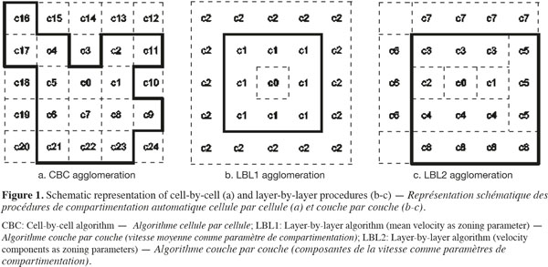
22At last, the agglomeration of the cells into zones could be realized by adding adjacent cells one-by-one (cell-by-cell, CBC) or by grouping all or part of the adjacent cells at the same time (layer-by-layer, LBL). A schematic description of these agglomeration procedures is presented on figure 1. Considering the LBL procedure, the adjacent cells to the growing zone can be added all together at the same time with respect to the tolerance (LBL1, Figure 1b) or by considering cells contiguous to each face of the new zone successively (LBL2, Figure 1c). In the case of the LBL procedure, cells are added when |P₀ - P_mean| < α.P₀, where P_mean is the mean value of P in the adjacent cells to be added.

3. Results

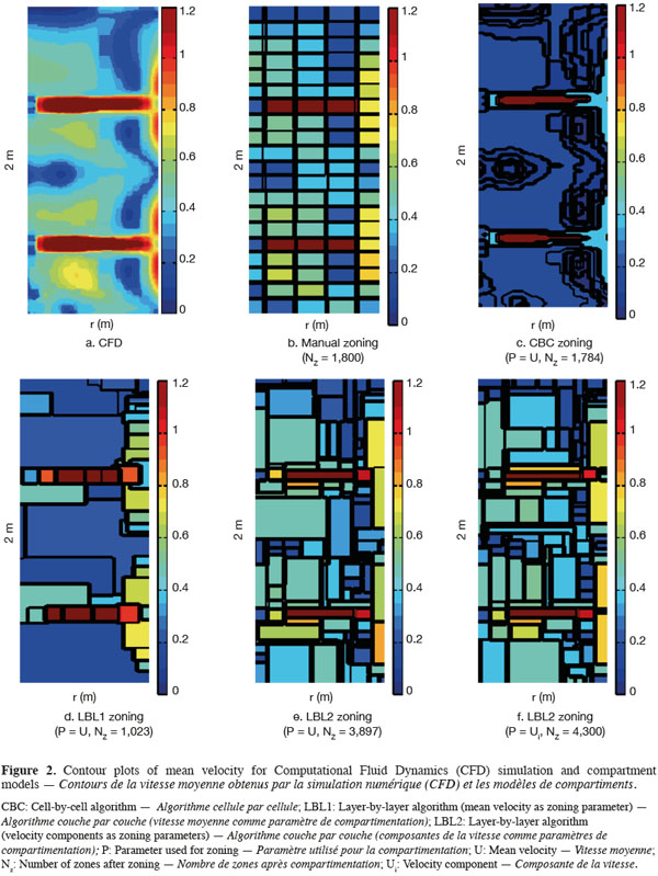
23On figure 2 are presented contour plots of the mean velocity on a vertical plane from CFD simulation (Figure 2a), manual zoning (Figure 2b), each automatic zoning procedure tested with mean velocity norm as agglomeration criterion (CBC, Figure 2c; LBL1, Figure 2d and LBL2, Figure 2e) and for the LBL2 algorithm with the three velocity components as agglomeration criterion (Figure 2f). The Y axis corresponds to the impeller axis and the black line on the contour plots represents the zone boundaries. The tolerance used for all automatic zoning algorithms is α = 0.5. For manual zoning, the tank is divided with a constant interval in each direction (ΔR = T/10, Δθ = π/9, ΔZ = H/20).

24In order to compare zoning procedures, the mixing of an inert scalar is simulated for CFD and each compartment model defined. A small volume of tracer is injected just below the liquid surface and near the tank wall. The computed mixing times are presented in table 1.

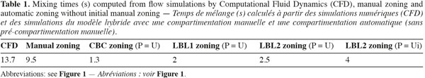
25The strong radial jet produced by Rushton impellers and the circulation loops above and below each impeller are quite well represented by all algorithms (manual and automatic), especially by the CBC and LBL1 algorithms (Figure 2). However, CBC and LBL1 algorithms tend to produce very large zones where velocity gradients are small, i.e. in the center of each circulation loop. As a consequence, the mixing time computed using the compartment models defined by CBC and LBL1 are significantly underestimated (Table 1). Increasing the number of zones using a smaller tolerance factor does not improve the mixing time results because the zone size is not significantly reduced in the bulk region. The LBL2 algorithm gives better results, especially when the three velocity components are chosen as agglomeration criterion. This algorithm produces a greater number of zones with the same tolerance criterion. This is due to the strong velocity gradients generated in the impeller region so that the zone size is very small and the number of zones is important in this region. As pointed out by Bezzo et al. (2004), the number of zones could be reduced by aggregation of the small zones in the impeller region without significantly modifying the mixing time computed.

26However, all mixing times computed from the automatic zoning models are underestimated compared to manual zoning or CFD. This can be explained by the size of the zones in the tangential (θ) direction. Indeed, for a given radius and a given height, mean velocities remain more or less constant in the tangential direction (axial symmetry), except around the baffles. So, the zones produced by the automatic zoning procedures are quite large in the θ direction.

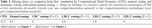
27To reduce the size of the zone in the tangential direction, an initial manual zoning is performed before the automatic zoning. It consists in dividing the tank volume in quarters according to the θ-coordinate. The size of each quarter is set to Δθ = π/9. Mixing times obtained with this method are presented in table 2. As can be seen from the mixing times, using an initial manual zoning before the automatic one improves the accuracy of the models. Despite that, CBC and LBL1 still underestimate significantly the mixing time. Manual and LBL2’ procedures predict well the concentration evolution. However, mixing times are smaller than those predicted by CFD and a time lag is observed between the concentration peaks predicted by CFD and by compartment models. The faster mixing predicted by compartment models can be explained by an insufficient number of zones.

4. Conclusion

28Hybrid CFD/compartment models can prove to be useful tools to predict the complex interaction between hydrodynamics and biological reactions in stirred-tank bioreactors. The focus of this work was to develop a methodology to define the compartments of such models from a CFD simulation. Several procedures have been tested and compared on the basis of mixing time computation. Both manual zoning algorithm and LBL2 automatic zoning algorithm based on the three velocity components and with an initial manual zoning enable to reproduce with a good accuracy the mixing of an inert tracer. The advantage of the automatic procedure lies in the fact that it can be used quite easily for other geometries. The difference observed between mixing times computed from CFD and compartment model simulations can be attributed to the restricted number of zones. Moreover, as the aim of the present paper was to develop an automatic zoning procedure, the influence of turbulence on the exchange fluxes between zones have not been taken into account. This could be done by computing a turbulent flow rate from the turbulent kinetic energy resolved by CFD.

Bibliographie

Pour citer cet article

A propos de : Angélique Delafosse

A propos de : Frank Delvigne

A propos de : Marie-Laure Collignon

A propos de : Michel Crine

A propos de : Philippe Thonart

A propos de : Dominique Toye