


- Accueil
- Volume 18 (2014)
- Numéro 3
- A review of inversion techniques related to the use of relationship matrices in animal breeding


Visualisation(s): 3289 (44 ULiège)
Téléchargement(s): 215 (2 ULiège)

A review of inversion techniques related to the use of relationship matrices in animal breeding

Notes de la rédaction
Received on September 9, 2013; accepted on February 14, 2014
Résumé
Synthèse bibliographique des techniques d’inversion impliquées dans l’utilisation de matrices de parenté en amélioration animale. En amélioration animale, les effets génétiques sont habituellement prédits par l’utilisation de modèles mixtes. Pour n’importe quel effet génétique, les modèles mixtes nécessitent l’inversion de la matrice de covariance associée à cet effet. Cette matrice est égale à la matrice de parenté associée, multipliée par le composant de la variance génétique également associé à cet effet. Étant donné la taille de nombreux systèmes d’évaluations génétiques, établir l’inverse de ces matrices de parenté peut s’avérer couteux d’un point de vue computationnel. Dans cette synthèse bibliographique, notre objectif est de passer en revue les techniques qui facilitent l’inversion de matrices de parenté utilisée en amélioration animale pour la prédiction des types d’effets génétiques suivants : effet additif, effet gamétique, effet dû à la présence de loci marqués de caractères quantitatifs, effet de dominance et différent effet d’épistasie. Les règles de construction de la matrice et les algorithmes d’inversion sont détaillés pour chaque matrice de parenté. Dans la discussion finale, nous esquissons un cadre théorique commun à la plupart des techniques d’inversion passées en revue. Deux contraintes computationnelles ressortent de ce cadre théorique : l’établissement de la matrice de dépendances entre niveaux de l’effet et celui de certaines parties (diagonales ou bloc-diagonales) de la matrice de parenté à inverser.
Abstract
In animal breeding, prediction of genetic effects is usually obtained through the use of mixed models. For any of these genetic effects, mixed models require the inversion of the covariance matrix associated to that effect, which is equal to the associated relationship matrix times the associated component of the genetic variance. Given the size of many genetic evaluation systems, computing the inverses of these relationship matrices is not trivial. In this review, we aim to cover computational techniques that ease inversion of relationship matrices used in animal breeding for prediction of the following different types of genetic effects: additive effect, gametic effect, effect due to presence of marked quantitative trait loci, dominance effect and different epistasis effects. Construction rules and inversion algorithms are detailed for each relationship matrix. In the final discussion, we draw up a common theoretical frame to most of the reviewed techniques. Two computational constraints come out of this theoretical frame: setting up the matrix of dependencies between levels of the effect and setting up some parts (diagonal or block-diagonal elements) of the relationship matrix to be inverted.
Table des matières
1. Introduction
1A simple model (equation 1; see Kempthorne, 1955) describes a given phenotype (P) as the sum of the genotype (G) and the environment (E) of a particular animal:
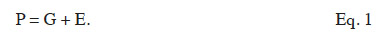
2Based on equation 1, variations among phenotypic observations are therefore explained by genetic and environmental variations and by a potential interaction between genotype and environment. Genetic improvement of animals requires accurate estimation of the genetic variance component in order to predict the genetic values of animals. The structure of this variance component is based on knowledge of the biological processes involved in Mendelian inheritance.
3In nearly all domestic species, animals have a diploid genome (with the exception of honey bees, where males are haploid). Then, during the production of gametes, a haploid copy of the diploid genome of the original animal (sire or dam) is made. However, haploid copies are produced from potentially different parts of the homologous chromosomes, following the process of recombination due to crossing-over. Thus, for any locus, a gamete carries a single copy of one of the two alleles carried by the parental genome. Both gametes eventually merge to create a new animal.
4By the process described before, every new animal has a specific and unique genetic makeup. Genetic covariances among different animals arise because they have inherited similar alleles and allele combinations. Based on these covariances, associations among these animals can be defined as ratios between covariances and variances associated to a given genetic effect. Whether the interactions between alleles of the same locus (intra-locus interaction) and between loci (inter-loci interaction) are null or not, several types of genetic effects can be distinguished. In our study, we will cover and detail the following genetic effects: additive, gametic, effect due to marked QTL, dominance and the different types of epistasis effects.
5When fitting a linear model with generalized least squares, use of the inverted covariance structure among observations allows obtaining Best Linear Unbiased Estimators. Prediction of genetic effects is usually obtained through the use of mixed models (Henderson, 1953; Henderson, 1973). These models are equivalent to models fitted using generalized least squares and, for every random effect, the inverse of the associated covariance structure is also needed.
6Due to huge size of regular genetic evaluations, there is a substantial interest in computational techniques that make efficient use of covariance matrices in terms of computing time and memory requirements. Thus, our main objective is to review and explain in detail algorithms for inversion of relationships matrices useful in animal breeding. Completion of this objective involved the definition of the relationships between levels of the concerned genetic effect and the computation of the related matrices for each type of genetic effect listed above (additive, gametic, marked QTL effects, dominance and epistasis). Finally, we outline a general framework of inversion of relationship matrices in the final discussion.
7It must be noted that the case of genomic relationship matrices has been willingly discarded in this study because no algorithm that directly sets up their inverses has been developed so far. The genomic relationships are made available by the use of dense marker chips (over than tens of thousands of markers) and give an accurate estimation of the observed relationship between two animals. For their computation, please refer to the work of VanRaden (2008), for additive genomic relationship matrix, and Su et al. (2012) for non-additive genomic relationship matrix.
2. Additive relationship matrix
2.1. Definition of the additive relationship
8If interactions between alleles are considered null, the genetic (co)variance is said to be “additive”. Based on previous work by Pearl (Pearl, 1917a; Pearl, 1917b), Wright (1922) defined an additive relationship coefficient as the additive correlation between two animals i and j (equation 2):
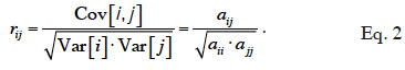
9The rij coefficient is a correlation coefficient; it ranges from 0 to 1. The non-scaled coefficient of Wright, noted aij, is the additive genetic relationship coefficient and, from equation 2, is defined as equal to rij √aii.ajj.
10This coefficient is also often referred as the “numerator relationship” coefficient (due to its position in equation 2). We will denote it as the “additive relationship coefficient” and the kind of relationship that it refers to as an “additive relationship” in our study. The matrix containing all these additive relationship coefficients will be denoted by A and called “additive relationship matrix”.
2.2. Computation of the additive relationship matrix
11Complete computation of the additive relationship matrix. The path coefficient method (Wright, 1922) enables the computation of the additive relationship between two animals. The process requires identification of all nearest ancestors shared between those two animals and counting of the number of generation steps between them. The path coefficient method can be automated and extended to computation of relationship coefficients in the whole population. The tabular method (Emik et al., 1949; Henderson, 1976) performs the computation of additive relationship coefficients in a recursive manner. For a given animal, the relationship coefficients of this animal with all older animals are computed in a row by adding one half of the relationship coefficients in the rows of its parents. A prior step is required: organization of pedigree records in a sorted by generation list of triplets animal-sire-dam (Emik et al., 1949; Mugnier et al., 1966). On a population of n animals, a square matrix of order n is created.
12This algorithm has a complexity that is proportional to n2, because, at each of the n loops it achieves, a linear combination of a vector of maximum length n is performed. Storage requirements follow the same trend and may quickly become prohibitive.
13Partial computation of the additive relationship matrix. For this reason, and also because only a section of the additive relationship matrix may be of interest in large populations, algorithms that permit a partial computation of the additive relationship matrix have been developed.
14Algorithms corresponding to two specific parts of the A matrix should be mentioned. The first one is an algorithm that computes the relationship coefficients of a particular animal with the rest of the population (e.g. Colleau, 2002). The second one is an algorithm that computes the diagonal elements of A, which reveals inbreeding coefficients (e.g. algorithms of Quaas, 1976; Meuwissen et al., 1992; Sargolzaei et al., 2005). The interest of these coefficients will be highlighted in the next sections.
2.3. Computation of the inverse of the additive relationship matrix
15Matrix A is non-singular except in the presence of genetically identical animals (GIA; full-twins or clones). In such situations, contributions of Kennedy et al. (1989) and Oikawa et al. (2009) are relevant.
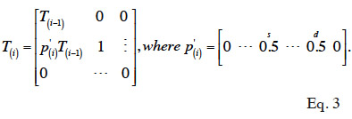
16In situations without GIAs, Henderson (1976) has proposed rules that allow computing the inverse of A without having to compute A explicitly. These rules are based on the simplicity of structure of matrices involved in the factorization of A: A = TDT’. According to Henderson (1976), matrix T can be computed recursively (equation 3): the vector corresponding to the i-th row of T, from column 1 to (i-1), is equal to one half of corresponding parental vectors (say s and d). Diagonal value is 1 and upper triangular part is 0.
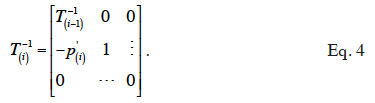
17Inverting the factorization of A and using it to compute the inverse of A (as (T-1)’D-1T-1) does not require T, but the inverse of T. This latter has a very simple structure that comes by inversion of a triangular matrix (equation 4):
18The matrix D is diagonal: element Dii is equal to
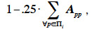
19where ∏i denotes the set of known parents (either 0, 1 or 2 parents known) of animal i. A correct computation ofD requires to know the diagonal elements of A. Algorithms for computation of inbreeding coefficients mentioned in section 2.2.2. are here of great interest. Among those, the algorithm by Quaas (1976) is noteworthy as it is the first one to compute these elements for the particular purpose of the computation of the inverse of A.
20Once matrix D has been computed, Henderson (1976) proposed a simple algorithm to set up the inverse (Algorithm 1). The algorithm summarizes the product (T-1)´D-1T-1) to n updates of a n-by-n matrix that was initially set to zero. Each update is a square block matrix of order 1 plus the number of known parents. This principle was demonstrated in Tier et al. (1993) and van Arendonk et al. (1994).
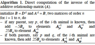
21The advantages of this algorithm are its low complexity (O(n)) and the low amount of memory required to store the very sparse output (A-1).
3. Gametic relationship matrix
3.1. Definition and uses of gametic relationships
In some situations, it may be interesting to express the additive genetic value of an individual in terms of the separate gametic contributions of each of their two parents (Kennedy et al., 1988; Schaeffer et al., 1989). Prediction of additive gametic values instead of additive genetic values allows reducing the size of the system to solve: the number of genetic effects is equal to the number of parents, necessarily lower than the total number of animals in the population. The covariance matrix used for random genetic (gametic) effects is called the “gametic relationship matrix” and denoted hereafter as Ga. Quaas et al. (1980) have developed such a model, known as reduced animal model. This model also shows how each ancestor affects the genetic value of the individual. Gibson et al. (1988) have proposed a gametic model in which only one parental gamete expresses the genetic effect (autosomally inherited) of an individual. Other uses are: analysis of haploid-diploids species such as the honey bee (Smith et al., 1985) and analysis of gametic imprinting effects (Gibson et al., 1988; Schaeffer et al., 1989). Eventually, the usefulness of the gametic relationship matrix in computation of the dominance relationship matrix has been shown by Schaeffer et al. (1989). The derivation of A from the gametic relationship matrix has been described by Smith et al. (1985) and showed by Jamrozik et al. (1991). Matrix A is obtained by 1/2KGK´, where 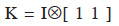 (Tier et al., 1993; van Arendonk et al., 1994).
3.2. Computation of the gametic relationship matrix
22Smith (1984) proposed an algorithm to compute Ga that is inspired by the tabular method (see section 2.2.1.). For diploids species, the size of the matrix will be N = 2n, where n is the number of animals in population. Each animal has thus two rows/columns that correspond to both parental gametes. Construction rules are simply deduced from the tabular method: if the parent p is known, then the row elements below diagonal are equal to the half of the sum of corresponding elements in both lines of parent p; else if the parent p is unknown, these elements are null. The corresponding column is obtained by transposition.
3.3. Inversion of the gametic relationship matrix
23Matrix Ga is non-singular within the same restriction as for matrix A (no clones).
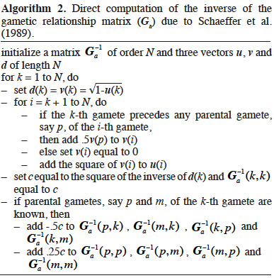
24The following algorithm (Algorithm 2) was developed by Schaeffer et al. (1989) based on direct computation of the inverse of A. Animals are supposed to be ordered chronologically. For each animal, the first and second gametes are respectively due to the sire and dam. Computation of the diagonal elements is similar to that of Quaas (1976).
4. Covariance matrices for marked QTL effects
4.1. Definition of marked QTL covariance
25Development of genetic engineering techniques leads to identify loci involved in determinism of quantitative traits (QTL) and to assist selection by use of markers linked to these QTL (Marked QTL, MQTL; Soller et al., 1983; Smith et al., 1986). The following model (Fernando et al., 1989) integrates effects of a causative QTL into BLUP.

26In equation 5, a phenotypic value yi is decomposed in environmental contributions xi´ß, random additive genetic contributions: a contribution of the paternally inherited allele of a marked QTL (vpi), a contribution of the maternally inherited allele of the same marked QTL (vmi ) and a residual additive contribution due to QTLs unlinked to the marker (ui), and a random error contribution (ei). Solving this mixed model requires the covariance matrix of the vi values (called “MQTL matrix” and denoted as G hereafter), which is computed using both pedigree relationships and marker information.
4.2. Computation of the MQTL matrix
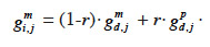
27Fernando and Grossman (1989) have developed the “MQTL relationship” in a similar manner as the additive relationship. While this latter is based on the probability that alleles at a same locus for each animal are IBD, MQTL relationship is based on the conditional probability of the same event given information on a marker closely linked to the MQTL. This conditional probability is affected by the recombination rate r between the marker locus and the marked QTL (outlined and developed similarly in Chevalet et al., 1984): given that an animal inherited the paternal marker allele of its sire, the probability that he also inherited the paternal QTL allele of its sire is (1-r) whereas the probability that he inherited the maternal QTL allele of its sire is r. The MQTL relationship between two animals i and j, for both paternal and maternal alleles (gpi,j and gmi,j), can thereby be computed recursively from the MQTL relationships between s, sire of i, and j (gps,j and gms,j) and d, dam of i, and j (gpd,j and gmd,j),
28given marker inheritance:
29– if i inherits from its sire its paternal marker allele:
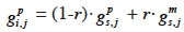
30– if i inherits from its sire its maternal marker allele:
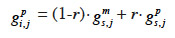
31– if i inherits from its dam its paternal marker allele:
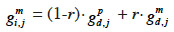
32– if i inherits from its dam its maternal marker allele:
33If no information on marker inheritance is available, then both paternal and maternal alleles have equal probability of being inherited and r is equal to 0.5. In such a case, the MQTL relationship is the corresponding gametic relationship. Matrix G has thus the same size as matrix Ga and, for computation purposes, is ordered in the same manner (parents before offspring; paternal allele before maternal allele). The computation goes through use of the recursive rules here above in a tabular method. van Arendonk et al. (1994) showed the recursion rule in matrix notation:
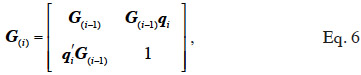
34where G(i-1) is the MQTL matrix for gametes 1 to i-1 and qi is a vector that has two non-zeros entries: (1-r) to the position of the parental gamete whose allele was inherited and r to the position of the other parental gamete. An algorithm by Wang et al. (1995) also follows an identical tabular method but processes animal by animal (thus, 2 lines/rows at a time) instead of gamete by gamete. The tabular method for constructing G is therefore:
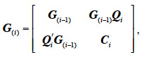
35where Ci is a 2-by-2 matrix with 1 on the diagonal and the inbreeding coefficient of animal i elsewhere and Qi is a 2-by-(i-1) matrix with maximum 8 non-zeros elements, in all 4 columns corresponding to the 2 parental gametes. These elements are filled with the probability of descent for each offspring QTL allele from any parental QTL allele. It is worth noting that this algorithm accommodates situations where paternal or maternal origin of alleles cannot be determined.
36A very similar algorithm was developed by Goddard (1992) for the covariance matrix between effects of potential QTL surrounded by two marker loci. In this algorithm, the relative position p of the QTL to the marker loci is used instead of the recombination rate of Fernando et al. (1989). Tracing inheritance of chromosome segments instead of marker loci enhances accuracy of the model. For genetic evaluation systems including many ancestors without marker information, Hoeschele (1993) showed that QTL effects were needed only for genotyped animals and common ancestors of these animals. Elimination of these equations led to a substantial reduction of the order of the covariance matrix. Such an algorithm that accounts for non-genotyped parents is also presented in Wang et al. (1995).
4.3. Direct computation of the inverse of the MQTL matrix
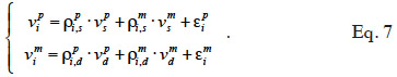
The algorithm of Fernando et al. (1989) follows the same approach as Henderson (1976) and Quaas (1976). Using a definition similar to that of their tabular method, they relate both effects of paternal and maternal MQTL (vpi and vmi) to their parental MQTL (vps, vms, vpd and vmd) effects in a simple linear model (equation 7). In this model, coefficients  allocate r or (1-r) accordingly with the inheritance turned up by marker information and
  and
and  residual effects, whose covariance matrix
  is shown to be diagonal.
37Assuming that inbreeding coefficients are available, the algorithm proceeds through the pedigree and fills in the inverse of the MQTL matrix (initialized to a null matrix of order N) in three steps:
– compute the diagonal element d of  as
as 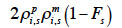
for a paternal gamete or as 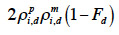
38 for a maternal gamete;
– set up a vector q equal to 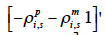
for a paternal gamete or equal to 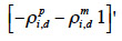
39 for a maternal gamete;
– add the product  to the inverse matrix to positions corresponding to each of its parental gamete and the current gamete itself.
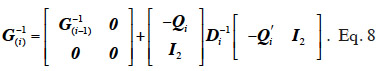
The algorithm by van Arendonk et al. (1994) is equivalent to the previous one and is outlined under the form of the successive blockwise inversion of Tier et al. (1993). It requires thus the computation of all MQTL relationships of the population. Equivalently, the algorithm of Wang et al. (1995) for direct computation of the inverse of the MQTL relationship matrix processes the two gametes of an animal at a time, as shown in equation 8 where 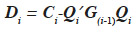 is the Schur complement of G(i-1) :
40Efforts in reducing computational costs of this algorithm have been outlined (Abdel-Azim et al., 2001; Matsuda et al., 2002; Tuchscherer et al., 2004). The computing cost reduction performed by Sargolzaei et al. (2006), applying the indirect method of Colleau (2002) to the MQTL matrix, is also of great interest.
4.4. Computation and inversion of a covariance matrix for an animal model accounting for MQTL relationships
The closeness between gametic and MQTL relationship matrices has already been mentioned. Also, it has been mentioned that the additive genetic relationship matrix A could be retrieved from the gametic relationship matrix using an incidence matrix K (see section 3.1.). Similarly, it is worth noting that a modified A (noted hereafter AM) could be obtained from the MQTL matrix (van Arendonk et al., 1994) as  Computation of the inverse is made successively in a similar manner as for G (see previous section). However, vectors qi have non-trivial values. Their computation is therefore made using a construction of AM similar to equation 6 for G. An analogous equation would express the i-th above diagonal column vector of AM (AM,i) as AM,i = AM,(i-1)qi. Therefore, vectors qi are obtained by the product qi = A-1M,(i-1)AM,j.
41This product can be interpreted as a linear regression of the relationships between the (i-1) first animals on their relationships with the i-th animal.
5. Dominance relationship matrix
5.1. Definition of dominance
42Dominance is defined by Fisher (1918) as the portion of the partitioned phenotypic variance that results from allelic interactions at the same locus. A dominance effect is the genetic effect carried on by a given allelic combination. When two animals share common ancestors, it becomes therefore likely that they carry an identical allelic combination. A dominance relationship coefficient scales this likelihood. Among others (epistasis effects), dominance is the non-additive genetic effect that is the more relevant in domestic species evaluation (Gengler et al., 1998).
43Dominance relationship coefficient dij between animals i (having parents s and d) and j (having parents p and m) can be obtained from the additive relationship coefficients by the formula (Henderson, 1985): dij = .25(asp adm + asm adp). The matrix containing all dominance relationship coefficients is denoted by D and is called the dominance relationship matrix.
5.2. Computation of the dominance relationship matrix
44Using formula above, D is computed using A. Also, a general recursion formula to compute D has been outlined in Smith et al. (1990). Note that both A and D can easily be derived from the gametic relationship matrix (see section 3).
5.3. Computation of the inverse of the dominance relationship matrix
45Because dominance is inherited through pairs of parents, two full-sibs have the same rows and columns in D and therefore D is not of full rank. To overcome this singularity, Hoeschele et al. (1991) partitioned the dominance effects into sire X dam subclass effects (and a within-subclass deviation due to Mendelian sampling). They developed an inversion algorithm that sets up the inverse of the covariance matrix (noted F) of sire X dam subclass effects. The individual dominance effects are then related to these subclass effects. A recursive rule exists to compute the subclass effects (f). If S and D denote the sire and dam of an animal, SS and DS, the parents of its sire, SD and DD, the parents of its dam, the S-D subclass effect (fS,D) is obtained by:
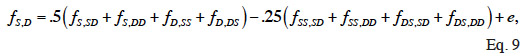
46where e is a segregation residual. Their method includes in three steps:
47– identification of all filled sire X dam subclasses (among 8 potential subclasses in equation 9) that provide relationship ties;
48– direct computation of the inverse of F (see Algorithm 3);
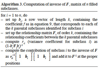
49– computation of the inverse of D using an incidence matrix that relates dominance effects to subclass effects.
6. Epistasis Matrices
6.1. Definition of epistasis
50Epistasis is a term that refers to interactions between loci (Bateson, 1909; Sinnot et al., 1950). Epistasis interactions used in animal breeding are (Cockerham, 1952; Cockerham, 1954):
51- the effect of a particular allele of a first locus on a particular allele of the second locus, additive by additive interaction (AXA);
52– the effect of a particular allele of a first locus on a particular allelic combination at the second locus (additive by dominance interaction, AXD), or;
53– the effect of a particular allelic combination at a first locus on a particular allelic combination at the second locus (dominance by dominance interaction, DXD).
54Other epistasis matrix can also be cited (additive by additive by additive, additive by additive by dominance, and so on; see Henderson, 1985).
6.2. Computation and inversion of the additive by additive relationship matrix
55The AXA relationship matrix, denoted by AA hereafter, can be formed rapidly by forming A using the tabular method and squaring each element (Cockerham, 1954; Kempthorne, 1955; Henderson, 1985; VanRaden et al., 1991).
56Chang et al. (1989) have developed a direct computation of the inverse of AA constructed using only sire and maternal grand-sire information. Their algorithm fills in the inverse matrix through a quick reading of the pedigree. However, the subclass effect sire X dam is included in the Mendelian sampling effect. VanRaden et al. (1991) have solved this drawback by setting up an algorithm that accounts for all subclass effects as for dominance (see equation 9). The relationships between AXA effects (u) are modelled by the linear relation u = Pu + Pbub + m, in which P and Pb are incidence matrices, ub is the vector AXA effects of unknown ancestors and ancestors combinations and m, the vector of AXA Mendelian sampling effects. After manipulations, the inverse of U, covariance matrix of u divided by the AXA variance component, can be expressed as (I-P´)R-1(I-P), where R is the covariance matrix of Pbub + m divided by the AXA variance component. An algorithm – similar to that for dominance, see Algorithm 3 – is proposed to compute the inverse of U. This algorithm proceeds as follows:
571. Identification of all AXA subclass effects, written in an expanded list. These subclasses include all animals and parental combinations that provide relationship ties. Therefore, the size of the AXA effects covariance matrix (U) may be several times the number of animal; this increased size is nonetheless offset by the resulting sparseness of its inverse.
582. Forward reading of the expanded list created at step (1). For each individual in this list, coefficients pertaining to the individual and its sire, dam and sire-dam subclass effect are added to U-1; for each sire-dam subclass, coefficients pertaining to that subclass and its ancestor subclasses are added to U-1. For both individual and sire-dam subclass, values and number of coefficients vary depending on the number of known sources.
59In an inbred population, the effects of sire, dam and sire-dam subclass are correlated and the values of coefficients are affected by inbreeding.
6.3. Computation and inversion of other epistasis matrices
60Others fore-mentioned epistasis matrices are computed similarly as the AXA matrix, by a Hadamard product of dominance and/or additive genetic matrices.
61Their inversion may be performed by classical inversion algorithms (Henderson, 1985; Palucci et al., 2007). A general methodological frame to solve a model including any epistasis effect (also, dominance effect) without inversion of the relationship matrix of this effect has been presented by Schaeffer (2003). This method computes solutions of the desired effects as a selection index from the additive genetic solutions and iteratively corrects the observations for these desired effects and computes additive genetic solutions until convergence is reached.
7. Discussion and conclusions
62A general framework for inversion of variance-covariance matrices of genetic effects may be drafted through the different kinds of genetic effects described and their associated relationship matrices.
The variance-covariance matrix of a genetic effect vector v is usually defined as the product (equation 10) of a relationship matrix, say W, and the genetic variance component associated to this effect, say 

63The vector v is modelled by a linear model: v = Bv + e, where B is an incidence matrix that gathers dependencies between elements of v and e is a term accounting for a residue due to the particular element itself (or, undue to dependencies between elements of v). It has to be noted that elements of v must be ordered such that any element only depends of elements preceding him; that is matrix B must be lower triangular. Removing recursion of this model returns v = (I-B)-1·e. Variance of v can thereby be expressed in terms of variance of the residual term (e; equation 11):

The covariance among residual terms is usually null, because these terms refer to the own specificity of the effect (individual, gamete or subclass). Consequently, the variance-covariance matrix of e is the product of a diagonal matrix, say D, by  Thereby, equating equations 10 and 11, it comes out that the relationship matrix associated to any of these described genetic effects can be expressed as W = (I-B)-1·D·(I-B´)-1, and a general expression of its inverse is:

64It worth noting that this expression is the inverse of the root-free Cholesky factorization of W, for which the lower triangular factor is (I-B)-1.
65It has been proposed (Henderson, 1976) and shown (Tier et al., 1993) that setting up the inverse of W using formula in equation 12 sums up to adding the contributions of a list of numbered levels of effect (individuals, gametes, subclass effects) to a null matrix. This successive addition can be achieved for x levels at a time. Usually, x is equal to 1 but may be greater than 1 in some situations (Smith et al., 1990; Wang et al., 1995; Sargolzaei et al., 2006).
66If we assume the following partitions for the relationship matrix W after i additions of x levels (W(i)) and the corresponding matrix B:
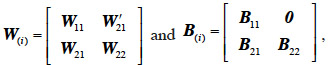
67then the i-th addition of x levels to the inverse returns the matrix W-1(i) :

68The computational step in equation 13 requires to know sub-matrices W22, W21 and B21.
69Therefore, we conclude by defining a computationally efficient algorithm for inversion of a genetic relationship matrix, on the basis of equation 13, as an algorithm that provides means to set up these sub-matrices (W22, W21 and B21) at a reduced computational cost.
70Setting up B21 often requires no computation because the dependency coefficients between levels of effects in v are a priori known (e.g. additive and gametic relationships). In some cases, e.g. MQTL matrices, few computations are required to set up these coefficients. Also, as shown by van Arendonk et al. (1994), these coefficients can be obtained by partitioned matrix theory. The original model of dependencies between levels in v can also be simplified by adding sub-levels, what enables to set up B21 more readily (Hoeschele et al., 1991; VanRaden et al., 1991).
71Setting up W22 and W21 is either implicit (e.g. gametic relationships and additive and dominance relationships of non inbred populations have all diagonal elements equal to 1), either requires explicit computation of the relationship matrix (e.g. MQTL matrices). In this second case (e.g. additive and dominance relationships of inbred populations and derived epistasis matrices), computation efficiency can be greatly enhanced using algorithms of partial computation of A (e.g. Quaas, 1976; Colleau, 2002).
72List of abbreviations
73AXA: additive by additive epistasis
74BLUP: best linear unbiased predictor
75DXD: dominance by dominance epistasis
76GIA: genetically identical animals
77IBD: identical by descent
78MQTL: marked quantitative trait locus
79QTL: quantitative trait locus
Bibliographie
Abdel-Azim G. & Freeman A.E., 2001. A rapid method for computing the inverse of the gametic covariance matrix between relatives for a marked Quantitative Trait Locus. Genet. Sel. Evol., 33, 153-173.
Bateson W., 1909. Mendel’s principles of heredity. Cambridge, UK: Cambridge University Press.
Chang H.L., Fernando R.L. & Gianola D., 1989. Inverse of an additive × additive relationship matrix due to sires and maternal grandsires. J. Dairy Sci., 72, 3023-3034.
Chevalet C., Gillois M. & Khang J.V.T., 1984. Conditional probabilities of identity of genes at a locus linked to a marker. Genet. Sel. Evol., 16, 1-13.
Cockerham C.C., 1952. Genetic covariation among characteristics of swine. PhD thesis: Iowa State College (United States of America).
Cockerham C.C., 1954. An extension of the concept of partitioning hereditary variance for analysis of covariances among relatives when epistasis is present. Genetics, 39, 859-882.
Colleau J.-J., 2002. An indirect approach to the extensive calculation of relationship coefficients. Genet. Sel. Evol., 34, 409-421.
Emik L.O. & Terrill C.E., 1949. Systematic procedures for calculating inbreeding coefficients. J. Hered., 40, 51-55.
Fernando R.L. & Grossman M., 1989. Marker assisted selection using best linear unbiased prediction. Genet. Sel. Evol., 21, 467-477.
Fisher R.A., 1918. The correlation between relatives on the supposition of mendelian inheritance. Earth Environ. Sci. Trans. R. Soc. Edinb., 52, 399-433.
Gengler N., Misztal I., Bertrand J.K. & Culbertson M.S., 1998. Estimation of the dominance variance for postweaning gain in the U.S. Limousin population. J. Anim. Sci., 76, 2515-2520.
Gibson J.P., Kennedy B.W., Schaeffer L.R. & Southwood O.I., 1988. Gametic models for estimation of autosomally inherited genetic effects that are expressed only when received from either a male or female parent. J. Dairy Sci., 71(Suppl. 1).
Goddard M.E., 1992. A mixed model for analyses of data on multiple genetic markers. Theor. Appl. Genet., 83, 878-886.
Henderson C.R., 1953. Estimation of variance and covariance components. Biometrics, 9, 226-252.
Henderson C.R., 1973. Sire evaluation and genetic trends. In: Proceedings of the Animal Breeding and Genetics Symposium in Honor of Dr Jay L. Lush. Champaign, IL, USA:American Society of Animal Science and The American Dairy Science Association, 10-41.
Henderson C.R., 1976. A simple method for computing the inverse of a numerator relationship matrix used in prediction of breeding values. Biometrics, 32, 69-83.
Henderson C.R., 1985. Best linear unbiased prediction of nonadditive genetic merits in noninbred populations. J. Anim. Sci., 60, 111-117.
Hoeschele I., 1993. Elimination of quantitative trait loci equations in an animal model incorporating genetic marker data. J. Dairy Sci., 76, 1693-1713.
Hoeschele I. & VanRaden P.M., 1991. Rapid inversion of dominance relationship matrices for noninbred populations by including sire by dam subclass effects. J. Dairy Sci., 74, 557-569.
Jamrozik J. & Schaeffer L.R., 1991. An equivalent gametic model for animal dominance genetic linear model. J. Anim. Breed. Genet., 108, 343-348.
Kempthorne O., 1955. The theoretical values of correlations between relatives in random mating populations. Genetics, 40, 153-167.
Kennedy B.W. & Schaeffer L.R., 1989. Genetic evaluation under an animal model when identical genotypes are represented in the population. J. Anim. Sci., 67, 1946-1955.
Kennedy B.W., Schaeffer L.R. & Sorensen D.A., 1988. Genetic properties of animal models. J. Dairy Sci., 71, 17-26.
Matsuda H. & Iwaisaki H., 2002. A recursive procedure to compute the gametic relationship matrix and its inverse for marked QTL clusters. Genes Genet. Syst., 77, 123-130.
Meuwissen T.H.E. & Luo Z., 1992. Computing inbreeding coefficients in large populations. Genet. Sel. Evol., 24, 305-313.
Mugnier M., Sutter J. & Goux J.-M., 1966. Organigrammes pour l’étude mécanographique de la parenté et de la fécondité dans une population. Population, 1, 75-98.
Oikawa T. & Yasuda K., 2009. Inclusion of genetically identical animals to a numerator relationship matrix and modification of its inverse. Genet. Sel. Evol., 41, 25.
Palucci V., Schaeffer L.R., Miglior F. & Osborne V., 2007. Non-additive genetic effects for fertility traits in Canadian Holstein cattle. Genet. Sel. Evol., 39, 1-13.
Pearl R., 1917a. The probable error of a Mendelian class frequency. Am. Nat., 51, 144-156.
Pearl R., 1917b. The selection problem. Am. Nat., 51, 65-91.
Quaas R.L., 1976. Computing the diagonal elements and inverse of a large numerator relationship matrix. Biometrics, 32, 949-953.
Quaas R.L. & Pollak E.J., 1980. Mixed model methodology for farm and ranch beef cattle testing programs. J. Anim. Sci., 51, 1277-1287.
Sargolzaei M., Iwaisaki H. & Colleau J.-J., 2005. A fast algorithm for computing inbreeding coefficients in large populations. J. Anim. Breed. Genet., 122, 325-331.
Sargolzaei M., Iwaisaki H. & Colleau J.-J., 2006. Efficient computation of the inverse of gametic relationship matrix for a marked QTL. Genet. Sel. Evol., 38, 253-264.
Schaeffer L.R., 2003. Computing simplifications for non-additive genetic models. J. Anim. Breed. Genet., 120, 394-402.
Schaeffer L.R., Kennedy B.W. & Gibson J.P., 1989. The inverse of the gametic relationship matrix. J. Dairy Sci., 72, 1266-1272.
Sinnot E.W., Dünn L.C. & Dobzhansky T., 1950. Principles of genetics. New York, USA: McGraw-Hill Book Co.
Smith C. & Simpson S.P., 1986. The use of genetic polymorphisms in livestock improvement. J. Anim. Breed. Genet., 103, 205-217.
Smith S. & Allaire F., 1985. Efficient selection rules to increase non-linear merit: application in mate selection. Genet. Sel. Evol., 17, 387-406.
Smith S. & Mäki-Tanila A., 1990. Genotypic covariance matrices and their inverses for models allowing dominance and inbreeding. Genet. Sel. Evol., 22, 65-91.
Smith S.P., 1984. Dominance relationship matrix and inverse for an inbred population. Columbus, OH, USA: The Ohio State University, Department Dairy Science, Mimeo.
Soller M. & Beckmann J.S., 1983. Genetic polymorphism in varietal identification and genetic improvement. Theor. Appl. Genet., 67, 25-33.
Su G. et al., 2012. Estimating additive and non-additive genetic variances and predicting genetic merits using genome-wide dense single nucleotide polymorphism markers. PLoS ONE, 7, e45293.
Tier B. & Sölkner J., 1993. Analysing gametic variation with an animal model. Theor. Appl. Genet., 85, 868-872.
Tuchscherer A., Mayer M. & Reinsch N., 2004. Identification of gametes and treatment of linear dependencies in the gametic QTL-relationship matrix and its inverse. Genet. Sel. Evol., 36, 621-642.
van Arendonk J.A.M., Tier B. & Kinghorn B.P., 1994. Use of multiple genetic markers in prediction of breeding values. Genetics, 137, 319-329.
VanRaden P.M. & Hoeschele I., 1991. Rapid inversion of additive by additive relationship matrices by including sire-dam combination effects. J. Dairy Sci., 74, 570-579.
VanRaden P.M., 2008. Efficient methods to compute genomic predictions. J. Dairy Sci., 91, 4414-4423.
Wang T. et al., 1995. Covariance between relatives for a marked quantitative trait locus. Genet. Sel. Evol., 27, 251-274.
Wright S., 1922. Coefficients of inbreeding and relationship. Am. Nat., 56, 330-338.
