1 Introduction

High-performance materials obtain their characteristic properties such as strength only by adapted production processes that control the microstructure in the material. Consequently, there is a need for numerical process simulations of production processes to predict the mechanical properties resulting from the manufacturing process.

In the automotive industry, the distributions of pre-strain, thinning and pre-damage as predicted by a numerical forming simu-lation are often taken as initial values for the crashworthiness analysis. Modern commercial simulation packages, such as LS-DYNA, are, thus, essential throughout the automotive development process. Their capabilities are not limited to this field.

For other industries, the numerical process simulation gains importance, too. Due to the small material yield in conventional processing of titanium alloys, e.g. Ti-6Al-4V, several innovative processes have been proposed recently. While the conventional processes lead to known material properties, this is not the case for processes such as additive manufacturing followed by hot isostatic pressing (HIP) [1] and combinations of AM and metal forming [2, 3]. The material properties of Ti-6Al-4V depend on the microstructure generated by phase transformations and evolution of internal variables such as dislocation densities and grain size.

In most commercial tools, tailored formulations for the phase transformation kinetics are only available for a limited number of processes and materials, like the hot stamping of the manganese-boron-steel 22MnB5 [4]. To overcome this limitation, the material model *MAT_254 / *MAT_GENERALIZED_PHASE_CHANGE provides a more general framework in terms of materials and processes in the commercial multi-physics FE-Solver LS-DYNA. It has been successfully been applied to, first, hot stamping and welding applications with steel alloys [5] and, second, to aluminum alloys [6]. Recent enhancements aim for process simulations with Ti-6Al-4V [7]. This material model allows working with up to 24 different phases, where it is up to the user to define the physical representation of each phase and the phase transformations to be considered. The resulting properties are obtained from the phase fractions and properties of each phase using a mixture rule.

Industrial process simulation is performed on the macroscopic (process) scale and therefor the morphology inside the material cannot be considered directly. Instead, so called internal variables are used to quantify the effects. This contribution shows a gen-eralized approach to include internal variables into macroscopic process simulations with LS-DYNA. Focus is put on necessary variables for Ti-6Al-4V, i.e., the evolution of phases, grain size and dislocation density. Other aspects such as precipitations and their morphology, can also be addressed by this approach, but is not of importance for Ti-6Al-4V.

The next section gives a short overview on *MAT_254, followed by a summary of the model of Bambach et al. [8] and its implementation into the material law. The application of this extended material on different test cases shows the functionality of the implementation in the third section.

2 Modelling Ti-6Al-4V with MAT_254 in LS-DYNA

2.1 Modelling Phase transformation kinetics

The commercial Finite Element Code LS-DYNA is used in a wide range of engineering problems. Due to its “one-code-strategy” it enables the users to easily simulate coupled problems like the thermo-mechanical forming processes. This includes phase trans-formations, which occur in materials such as steel and titanium alloys, with the LS-DYNA material model *MAT_254 / *MAT_GENERALIZED_PHASE-CHANGE. Fig. 1 shows the LS-Dyna input structure for this material.

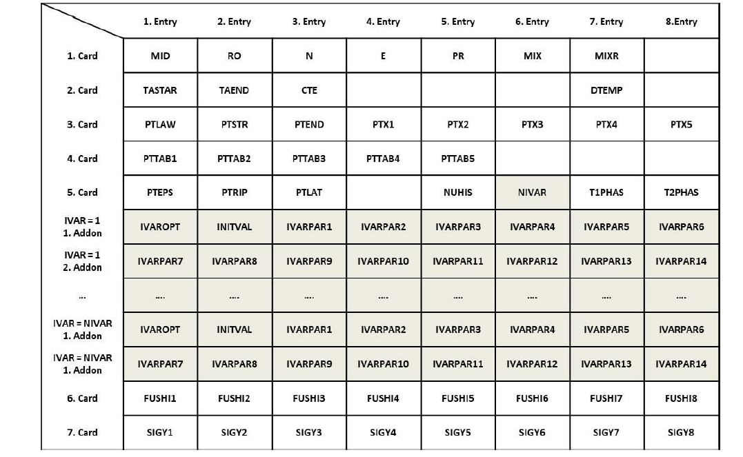
Fig. 1. LS-DYNA input for *MAT_254 including internal variables, the grey shaded entries relate to the new implementations

Beside standard input quantities in the first card, there is an additional parameter 𝑁 for the number of phases to be given, where up to 24 phases are currently supported. The sum of all phase fractions 𝑥𝑖 is equal to one. The parameter MIX specifies the initial mixture of the phases and MIXR the mixture rule to determine the mechanical properties. Per default, all mechanical properties are calculated by a linear combination:

where P is an arbitrary property and 𝑥𝑖 denotes the concentration of phase 𝑖.

The second card controls the annealing algorithm, accounts for thermal expansion, and defines a form of internal sub-cycling to resolve non-linear effects. As none of these features is used here, the respective parameters are not discussed.

The third and fourth cards specify the phase transformation models. Parameter 𝑁 influences the shape of the data referred to by the parameters in card 3 and 4 as it determines the input structure to be a 𝑁 by 𝑁-matrix, which is read by the material model as “from phase … to phase …” as is shown exemplarily in Fig. 2 (a) for 𝑁=4. In LS-DYNA, this is realized with a 2D-table, where the abscissae are the entries for the “starting phase” and the ordinates are load curves. The abscissae of any referenced load curve represent the “target phases” and the ordinates the respective transformation parameter.

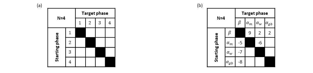
Fig. 2. (a) Generic input matrix for N=4, (b) phase transformation laws in matrix form for Ti-6Al-4V

The parameter PTLAW on the third card refers to such a matrix. It contains information between which of the 𝑁 phases transformations can occur during cooling, heating or both and determines the employed transformation model. A blank matrix entry corresponds to “no transformation”, whereas non-zero entries are connected to some pre-defined transformation model. Entries of “1”, ”3” and “4” are associated with the press hardening of 22MnB5. Entries of “2” and “12” represent generalized Johnson-Mehl-Avrami-Kolmogorov (JMAK) kinetics [5].

Of particular interest are the transformation laws associated with the values of “5”, “6”, “7”, “8”, and “9”, which are tailored for Ti-6Al-4V. The implementation follows the modelling approach presented by Charles-Murgau et al. [9,10] and Klusemann and Bambach [11] and has been validated in a previous contribution [5]. As sketched in Fig. 2 (b), four phases are defined (N=4) in the case of Ti-6Al-4V. They can be identified as 𝛽-phase, martensitic/massive 𝛼, Widmannstätten 𝛼, and grain boundary 𝛼, respectively. Recovery of the 𝛽-phase and Widmannstätten 𝛼 from martensitic and massive 𝛼 in heating conditions are described by transformation models “5” and “6”. The successive parabolic dissolution from the 𝛼-phases into 𝛽-phase during heating is controlled by the transformation models “7” and “8”. When the material cools down, the 𝛽-phase is transformed into the different 𝛼-phases. This is modelled by an extended Koistinen-Marburger approach (“9”) and a JMAK approach (“2”), respectively.

2.2 Yield stress computation in hotforming conditions for Ti-6Al-4V

By default, the yield stress is calculated by a linear mixture rule as in (1). Thus, the overall yield stress 𝜎 depends on the current phase fractions 𝑥𝑖 and the current values of the yield stresses 𝜎𝑖 of the individual phases:

The values of phase contributions 𝜎_𝑖 are functions of plastic strains, strain rates and temperature. Particularly, this last assumption is not justified for Ti-6Al-4V in hot forming conditions according to [8] and [12]: the yield stress contributions of 𝛼- and 𝛽-phases show a more complex behavior depending on strain, strain rate, temperature, and most important the deformation history. The latter is captured with internal variables such as fraction of globular 𝛼-phase 𝑋 and dislocation density 𝜌. The implementation shown in this contribution follows the approaches introduced in [8]. This section summarizes the yield stress definition introduced in [8] and relates it to the implementation in the material model *MAT_254.

Modelling compound materials knows two extrema, which can be interpreted either as a series connection (uniform stress model) or a parallel connection of springs (uniform strain model), representing the compounds. As the uniform strain model essentially leads to a linear mixture rule for the yield stresses as in (1), only this model is discussed in this contribution:

with 𝜎_𝛼 and 𝜎_𝛽 being the yield stresses of the 𝛼- and 𝛽-phases and their fractions 𝑓_𝛼 and 𝑓_𝛽. With the phase mapping shown in Fig. 2 (b) comparison of (2) and (3) allows for the following identifications:

Neither 𝜎_𝛼 nor 𝜎_𝛽 as defined in [8] fit into the standard description for the yield stress of a phase as provided by *MAT_254 and, consequently, an enhancement of the material model is needed to simulate hot forming applications with titanium. The contri-bution 𝜎_𝛽 is derived from experiments above the 𝛽-transus temperature, where only 𝛽-phase is found. It results in a phenomeno-logical model, cf. [13], that reads as follows:

Both stress contributions 𝜎_1𝛽 and 𝜎_2𝛽, are functions of an equivalent strain quantity 𝜀 and the Zener-Hollomon parameter 𝑍, which introduces a dependence on the strain rate 𝜀 ̇ and the temperature 𝑇 by its definition:

For the complete and rather lengthy expressions of 𝜎_1𝛽 and 𝜎_2𝛽 the reader is referred to the literature [8]. They are of no particular importance for the updates of the material model presented here. Instead of implementing the specific equations for 𝜎_1𝛽 and 𝜎_2𝛽, a flexible interface has been used for the yield stress definition. For each contribution 𝜎_𝑖, the user can now directly input the analytical equations. This is realized with the LS-DYNA keyword *DEFINE_FUNCTION that accepts arithmetic expressions as well as subroutines in the C or Fortran programming language. The material state variables such plastic strain, strain, strain rate, and temperature are handed to the *DEFINE_FUNCTION as independent variables.

This flexible approach can also be used to define the yield stress 𝜎_𝛼 for the 𝛼-phases. However, the definition adopted from [14], requires additional enhancements. The yield stress is assumed to be a combination of a thermal stress contribution 𝜏^∗ and an athermal stress contribution 𝜏_𝜇:

with 𝑀 being the constant Taylor factor. The thermal part 𝜏^∗ is a function of strain rate 𝜀 ̇ and the temperature 𝑇 and can, thus, be defined with the new reference to an analytical expression as discussed above. For the algebraic expression of 𝜏^∗, the user is referred to [8]. The athermal stress 𝜏_𝜇 requires further discussion as it is the result of different hardening mechanisms:

where 𝜏⁰ is the mechanical threshold stress, 𝛼₂ a material constant, 𝐺 the shear modulus, 𝑏 the magnitude of the Burgers Vector, 𝜌 the dislocation density, 𝐾_𝐻𝑃 the Hall-Petch coefficient and 𝐿 the average lath thickness of 𝛼-platelets.

In Eq. (9), the second term can be interpreted as work-hardening effect and the last term as grain size effect. These hardening effects naturally depend on deformation and temperature histories. Consequently, evolution equations must be defined for disloca-tion density 𝜌 and Hall-Petch coefficient 𝐾_𝐻𝑃. The material formulation for *MAT_254 has been extended to account internal variables that are associated with evolution equations. In the current implementation up to four internal variables can be established. Details on the input and implementation are given in section 2.3.

It clearly follows, that the current values of the internal variables are necessary for the yield stress calculation and are, thus, provided for the user-defined expression of the flow stress in the keyword *DEFINE_FUNCTION. The complete list of arguments for the function contains current time 𝑡, equivalent plastic strain 𝜀^𝑝, rate of equivalent plastic strain 𝜀̇^𝑝, equivalent strain value 𝜀, rate of the equivalent strain 𝜀̇, shear modulus 𝐺, bulk modulus 𝐾_𝑏𝑙𝑘, and, finally, quantities of the internal variables 𝑦₁, 𝑦₂, 𝑦₃, and 𝑦₄ if defined.

2.3 Internal variable definition in *MAT_254

The material input card in Fig. 1 represents the status of the material implementation. Parameters associated with the recent changes are highlighted. Parameter NIVAR defines the number of internal variables, but only up to four internal variables can currently be considered. For each internal variable, two additional lines of input are required.

The first additional entry IVAROPT defines the evolution equations to be used for the calculation. Five options for IVAROPT are available:

• “1” – use a *DEFINE_FUNCTION (a user defined function)

• “2” – use a grain size calculation for 22MnB5 (like in *MAT_244/248 in LS-DYNA)

• “3” – calculates the percentage of globular 𝛼-phase in Ti-6Al-4V, as in [8]

• “4” – calculates the dislocation density in Ti-6Al-4V, as in [8]

• “5” – calculates the Hall-Petch coefficient in Ti-6Al-4V, as in [8]

Option “1” offers the most flexibility and option “2” is tailored for UHS steels. In the following paragraphs, options “3”, “4” and “5” will be discusses in some detail as these are connected to the hot-forming of Ti-6Al-4V. The meaning of the evolution parameters IVARPAR1 to IVARPAR14 in the input depends on the choice of IVAROPT. In the following, the notation 𝜅_𝑖 is used in the equations for the 𝑖-th parameter IVARPARi to shorten the expressions.

2.3.1 Fraction of globular α-phase (IVAROPT=3)

Although the flow stress in (6) only contains the internal variables 𝜌 and 𝐾_𝐻𝑃, there is an implicit dependence on a third internal variable, namely the volume fraction of globularized 𝛼-phase 𝑋. Its evolution interacts with the evolution of the dislocation density.

Computation is invoked with IVAROPT=3 and starts with determining the critical strain 𝜀_𝐶 needed for the start of the globularization:

where the parameter 𝜅₄ can be interpreted as ratio of an activation energy 𝑄 and the universal gas constant 𝑅: 𝜅₄=𝑄/𝑅. If this critical value is exceeded, globularization follows an ordinary differential equation (ODE) with initial value 𝑋₀ that is input as parameter INITVAL. The ODE depends on strain 𝜀, strain rate 𝜀̇, material constants 𝑐₀,𝑐₁,𝑐₂, the average 𝛼-plate thickness 𝐿, the grain boundary mobility 𝑀_𝑏, and the activation force per unit area 𝑃, resulting in

It is important to note that mobility 𝑀_𝑏 and activation force 𝑃 are not constants but functions of temperature 𝑇, shear modulus 𝐺 and even of the dislocation density 𝜌. The actual expressions for 𝑀_𝑏 and 𝑃 are omitted here and can be found in [8]. Introducing the expressions into (11) and merging the material constants, the following form of the evolution equation can be obtained, which is used in the material model:

The dislocation density 𝜌 is not an intrinsic parameter of the material model, but it needs to be defined as internal variable as described in the following subsection. Therefore, additional information is needed for evaluation of (12). Parameter IVARPAR12 thus corresponds to the identification number of that internal variable that represents the dislocation density.

2.3.2 Dislocation density (IVAROPT=4)

The work hardening part in (9) mainly dependents on the dislocation density 𝜌. The initial value 𝜌₀ is defined by the second entry INITVAL of the first additional line. For the evolution equation that is activated by IVAROPT=4, a critical strain 𝜀_𝐶 again plays a role. It is calculated using (10) and enters the evolution equation for 𝜌, which reads [8]:

The previous equation shows that the evolution explicitly depends on globularization fraction 𝑋. The parameter IVARPAR12 determines the identification number of the internal variable "globularization fraction". Finally, the parameter 𝑘₂ in (13) depends on temperature and strain rate:

The parameter 𝜅₉ can be interpreted as ratio of an activation energy 𝑄 and the universal gas constant 𝑅: 𝜅₉=𝑄/𝑅. Furthermore, it is worth mentioning that in [8] the same activation energy value has been used for the critical strain in (10) and for the parameter 𝑘₂ in (19), equivalent to choosing 𝜅₄=𝜅₉.

2.3.3 Hall-Petch coefficient (IVAROPT=5)

The final term in (9) represents the size effects of the microstructure. The Hall-Petch coefficient 𝐾_𝐻𝑃 is calculated as internal variable for IVAROPT=5. Unlike globularization and dislocation density, the coefficient 𝐾_𝐻𝑃 cannot be directly expressed with a differential equation. In this case, an ODE can be provided for a coefficient 𝜆 as

with a steady-state value of 𝜅₂.The initial value 𝜆₀ is usually 1.0 and is defined by parameter INITVAL.

The Hall-Petch coefficient is proportional to 𝜆 and, furthermore, depends on the shear modulus 𝐺, the strain rate and the tem-perature. Merging the different coefficients, the Hall-Petch coefficient results in the following expression used in the material model:

3 Validation examples

Developments shown in this contribution closely follow the approach presented by Bambach et al. [8], where the predicted flow stresses are given for different constant temperatures and strain rates. For comparison, single element models are subjected to constant temperatures and displacement-controlled uni-axial loading with constant velocities.

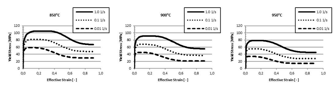
Fig. 3. Predicted flow stress for the 𝛽-phase at different strain rates and temperatures

First, only the 𝛽-phase is considered because this allows to validate the new interface to user-defined flow-stress input, by defining SIGY1 to refer to a function representing 𝜎_𝛽 in (6). Fig. 3 shows, that the new yield stress interface agrees precisely with the reference, proofing the validity of the implementation.

Each 𝛼-phase uses the same yield stress definition. Thus, parameters SIGY2, SIGY3, and SIGY4 refer to the same function id representing 𝜎_𝛼 in (8). As required by the expression, three internal variables are defined (NIVAR=3), for globularization, disloca-tion density and Hall-Petch coefficient, respectively. The flow curves predicted by the model are shown in Fig. 4. They show a perfect qualitative agreement with the reference and a very good quantitative fit. Parameters, which are not stated in [8], were estimated for the presented results and explain the minor differences.

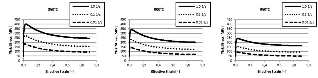
Fig. 4. Predicted flow stress for the 𝛼-phase at different strain rates and temperatures

Finally, the features of *MAT_254 for phase evolution kinetics and flow stress prediction are combined. Assuming an initial mixture of 𝛼_𝑚 (10%), 𝛼_𝑤 (88.5%) and 𝛽 (1.5%), elements are heated within 120s to 850°C, 900°C and 950°C, respectively. Fig. 5 (a) exemplarily shows the phase evolution during heating to 950°C. Flow stress results for combined 𝛼- and 𝛽-phase for the different temperatures at a strain rate of 1/s are given in Fig. 5 (b). Again, the results are in good agreement to the literature reference [8].

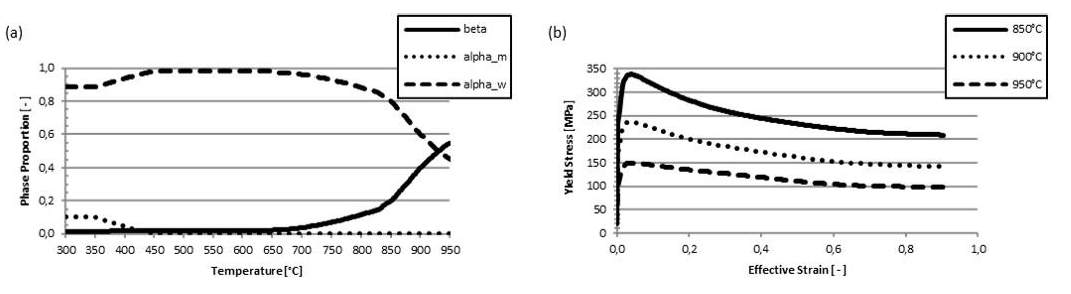
Fig. 5. (a) Predicted evolution of phases during heating from 300°C to 950°C, (b) resulting flow stress at strain rate of 1/s at different temperatures after heating

4 Summary and Outlook

In this paper recent developments for the LS-DYNA material *MAT_254 have been introduced. A new, flexible interface for flow stress definition and the concept of internal variables to capture the morphology of the microstructure have been discussed. A validation example has demonstrated that these features allow predicting the flow stress of Ti-6Al-4V in hotforming conditions in agreement with the literature.

For low temperatures, the standard plasticity algorithm based on an equivalent plastic strain measure and the temperature in *MAT_254 is feasible to describe flow behavior of Ti-6Al-4V. It seems reasonable to switch from one formulation to the other at a certain critical temperature range. Further improvements in calibration can be done with experimental investigations of static globularization [15] and microstructure properties of Widmannstätten and martensite at room temperature, as described in Fan et al. [16].

The validity of this approach for complex processes such as hybrid forming and welding applications like [17] will be the subject of further investigations.

Acknowledgments

The authors would like to thank Joanna Szyndler for providing validation curves.