1 Introduction

Predicting the deformation behavior of amorphous PET at elevated temperature is one of the most important problems in order to achieve accurate Stretch Moulding simulations (SBM). For decades, several material constitutive models have been proposed by researchers to describe the mechanical behavior of PET, particularly just above the glass transition temperature region which is the most critical temperature region for industry production, such as Boyce’s 3D model[1][2], ‘Glass-Rubber’ model from Buckley and Jones[3][4], augmented Buckley’s model proposed by Yan[5] and visco-hyperelastic model proposed by Chevalier et al[6].

Although researchers have spent lots of time on the constitutive relationships, there are weaknesses in their equations due to the fact that the deformation behavior of PET during deformation is extremely nonlinear and is influenced by many parameters, such as temperature, initial strain, deformation mode, stretch ratio, strain history and strain rate, as highlighted by Menary[7]. As a result, constitutive laws need to consider the effects of all these parameters, which makes modelling PET behavior become a very complex task. However this task is also suitable for ANNs which are able to overcome these problems that are difficult to be modeled by conventional mathematics and analytical methods[8].

Applications of ANNs can mainly be separated into 2 groups. In the first group, ANN are able to investigate the relationship between process parameters (such as heat treatment) and post processing properties (such as Young’s modulus). The second group focuses on building up an ANN-base model which can be used as a constitutive model implemented in FE code, which have already been used in some engineering applications , such as fiber polymer area[9] and metal forming area[10]. Once an ANN is trained perfectly, the neurons’ weights and biases will be extracted into a matrix which will be implemented into the user-defined material subroutine (VUMAT) as part of a constitutive model used during FEA forming simulation.

This paper aims to build up a model by ANN to predict the behavior of amorphous PET at conditions relevant to Stretch Blow Monlding i.e. Equibiaxial deformation in the temperature range 85℃ to 110℃ and strain rate range 1 s^-1 to 32 s^-1. The whole modelling process can be separated into 4 steps, as shown in Fig. 1.

Fig. 1. Flow chart of Artificial Neural Network

The first step is discussed in Section 2 of this paper whilst section 3 mainly focus on pre-training and training steps. The final step ‘Implement in FEA’ will be introduced in Section 4 of the paper.

2 Collect Data

2.1 Material characteristic

The PET sheet used in this work is supplied by DAK Americas as described by Yan[5].

Thermal properties take up a vital role in the experiments, which are determined by Yan et al [5] by Dynamic Mechanical Thermal Analysis (DMTA) and Differential Scanning Calorimetry (DSC). According to Yan’s results, the glass transition temperature(T_g) was 77℃, Cold crystallization occurs at 140℃ and the material begins to melt at 232℃.

2.2 Biaxial tension experiment

In the current paper, these experiments are carried out by Queen’s University Belfast’s Biaxial stretcher (QBS) which has already been introduced by Menary[11]. Experiments are separated into 6 temperature (T) groups from 85-110℃. In each temperature group, specimens are stretched equal biaxially to breaking point at 6 different strain rates (𝜀̇) ranging from 1 s^-1 to 32 s^-1. All experimental parameters are shown in Table 1. A selection of the Stress versus Strain curves are shown in Fig. 2.

Table 1. Strain rates & Temperatures used in biaxial stretch experiments

Fig. 2 (a) shows the influence of T at a strain rate of 4 whilst Fig. 2 (b) shows the influence of strain rate at a temperature of 100℃. It can be clearly seen that the σ-ε behavior is nonlinear viscoelastic with strong dependence on T and 𝜀̇.

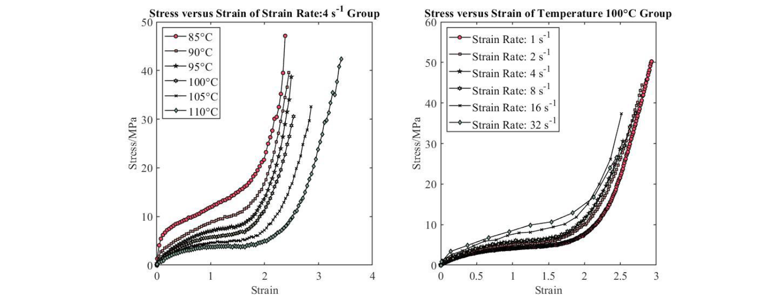
Fig. 2. Experimental σ-ε data showing influence of temperature at a strain rate of 4 s-1(a) and (b) showing influence of 𝜀̇ at a temperature of 100°C

3 Artificial Neural Network (ANN)

The characteristics of different notations will be shown by different letters. Scalars are represented by small italic letters: a,b,c; Vectors by small bold nonitalic letters: a,b,c; 2D Matrices are capital BOLD nonitalic letters: A,B,C

3.1 Introduction of Artificial Neural Network

The basic structure of the ANN is shown in Fig. 3, and a is calculated by (1).

Fig. 3. The basic structure of ANN

Where p is an input, known as scalar weight, b is known as bias. p, w and b will be inputted into the ‘Summer (Σ)’ in order to get the output n, which will pass to the transfer function or activation function (𝑓). A well-trained ANN usually consists of tens of or even hundreds of the basic structure shown in Fig. 3. The main task during training is to find out suitable values of w and b, which can describe the relationship between Input signal and Output signal accurately.

3.2 Select ANN architecture

The details of the ANN’s architecture used in this paper is shown in Fig. 4. According to Hagan et al [12], Irie and Miyake[13], 2 hidden layers perceptron is able to approximate any nonlinear function, as a result, the ANN used has 2 hidden layers which is indicated in Fig. 4 . Each hollow circle represents a neuron which is calculated by (1) and includes all structures shown in Fig. 3. Fig. 5 shows this architecture and the size of each matrix or vector notion including in Fig. 4.

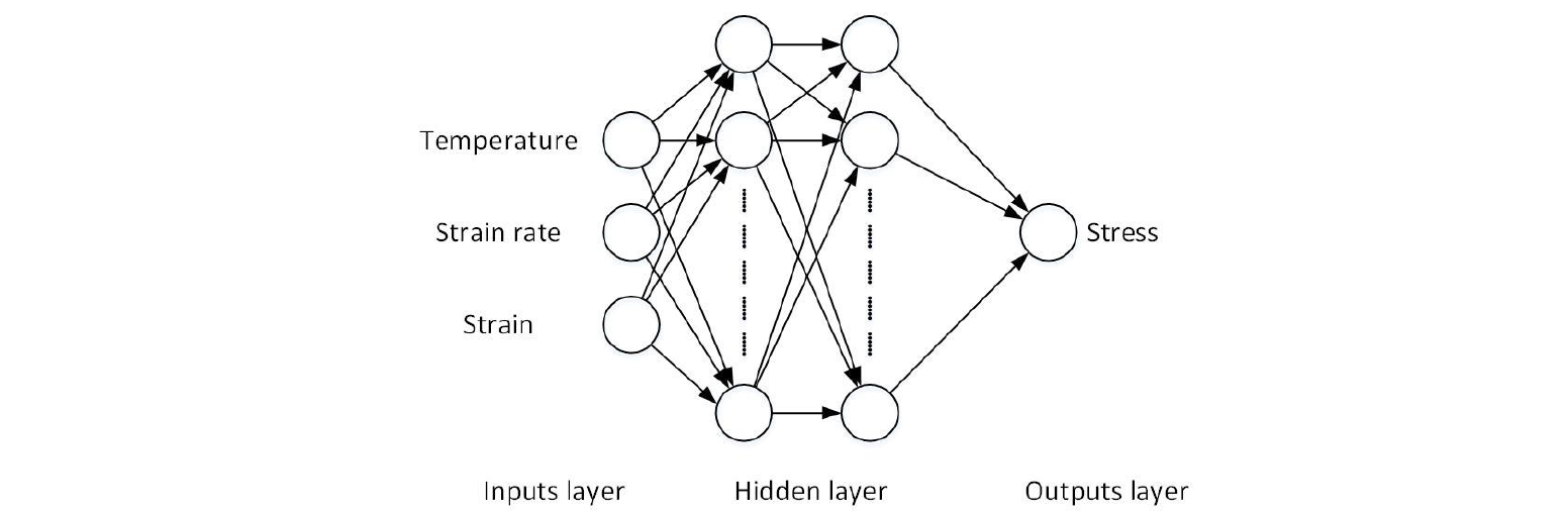
Fig. 4. Schematic illustration of the ANN structure

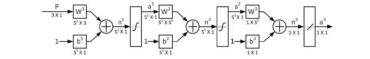
Fig. 5. Relationship between inputs/outputs vectors and weights/biases matrixes

Where P is known as an input vector which for this case contains temperature, strain rate and strain as shown in Fig. 4; Wⁱ and bⁱ are the weight matrix and biases vectors located in the i^th layer; aⁱ is the output vectors of the i^th layer. Sⁱ represents the size of column or row of Wⁱ.

There are two kinds of transfer functions used in Fig. 5, the first one is called ‘tansig’ function, which is represented by

And its mathematical expression is shown in

The second transfer function is ‘purelin’ function. This function is represented by

Its expression is shown in (3).

In addition to these two functions, several transfer functions can also be selected by researchers, such as Symmetric Saturating Linear function, Log-sigmoid function and competitive function[12]. The choice of these functions is influenced by lots of factors, for example the size of database, the distribution of data and the architecture of ANNs, so that the selection of transfer functions should be determined according to specific problems. According to Jordan et al [14] Al-Hail et al[15], the combination of ‘tansig’ function and ‘purelin’ function is capable to capture the Stress-Strain curves under biaxial tension experiments. In addition to these functions, the Log-sigmoid function is one of the most common choices for researchers, as shown in (4).

3.3 Training ANN

The training procedure is carried out by MATLAB and MATLAB Neural Network Tooling box[16]. The main training process starts with a loop which decides the initial architecture of the ANN before Bayesian Regularization following AI-Haik, Hussaini and Garmestani’ s method[15]. Exhausting Searching Method is carried out to find the architecture in the loop. This method is also adopted by Hussaini and Garmestani et al[15] and Jordan et al[14]. In the current works, Exhausting Searching Method starts with an [3,3] ANN ([3,3] stands for an ANN with 3 neurons in the first layer and 3 neurons in the second layer) and end up with [60,60] ANN. During Exhausting searching procedure, it increases 3 neurons on the first or second layers during each loop and records the ANN system’s performance. The performance of ANN is judged by Mean Square Error (MSE), E, which is shown as (5)

Where 𝑞 is the total number of inputs, 𝑖 is the order of every input, 𝑡_𝑖 is known as the target of ANN and 𝑎_𝑖 is the actual output of ANN.

The choice of increment during each iteration (3) and starting & ending point ([3,3]&[60,60]) is as same as the option of AI-Haik et al because the complexity of our database is similar. These 3 values are mentioned as empirical values in their work.

Due to AI-Haik, Hussaini and Garmestani’s work [15], iteration epochs is set to 500. According to Zhang [17], if MSE is less than 2.5x10^-2 , the ANN will be considered a high quality. In the current work the preferred error tolerance is 6×10^-3. This number is just an empirical value, obtained by referring to Zhang et al [17] and Hussaini et al [15]. With the increase of the number of neurons in both layers, the MSE decrease rapidly. As expected, the highest value of MSE appears when using a [3,3] ANN which is 1.238, whilst the [60,60] ANN shows the highest accuracy with a MSE of 0.005392 . However the [60,60] ANN also has the highest possibility of ‘Overfitting’ phenomenon. An ANN with 39 neurons in the first layer and 33 in the second layer ([39,33]) was the simplest structure which met the requirement of the error tolerance of 6x10^-3. As a result, [39,33] ANN will be used as the initial ANN of the Bayesian Regularization Algorithm.

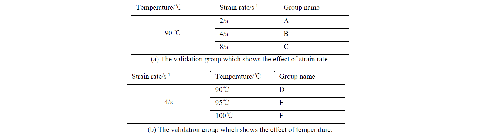
The Data was separated into two groups, one for training the ANN and another for validation. The data used for validation is shown in Table 2. In order to make sure, these validation groups are located in the training region, half of each group was chosen randomly for training during the training step.

Table 2. Data set for validation

4 Result and discussion

Prediction results of Group A, Group B and Group C are shown in Fig. 6. Generally, prediction results and experimental results fit very well in all groups. This figure indicates that current ANN model is able to predict strain-stress model in various strain rates with high accuracy.

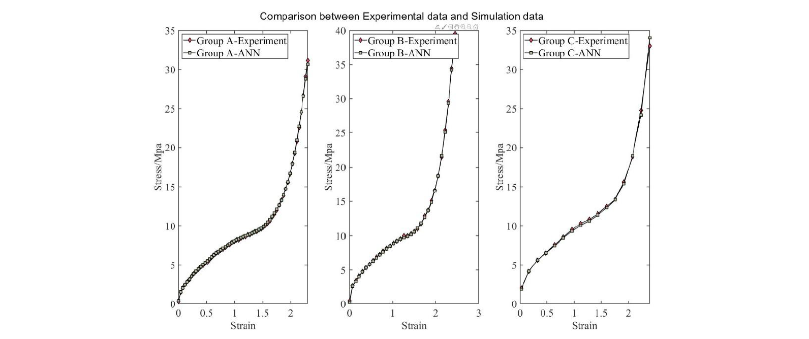
Fig. 6. Comparison between Experimental data and Simulation data in: 1) Group A:90°C,2/s; 2) Group B:90°C,4/s; 3) Group C:90°C, 8/s

The mean square error function is also used to judge results’ accuracy. The corresponding result is shown in Table 3. Table 3 shows that with the increase of the strain rate, the accuracy of prediction decrease slightly. This trend is caused by the number of data point of Force/displacement from the tension machine in different groups. According to Yan’s thesis [9], during biaxial extension experiments, strain and stress are recorded at a constant time interval (0.01s). If the strain rate is high, such as 8/s, the time to record the data is significantly reduced resulting in only 32 datasets compared to 118 datasets for 𝜀̇=4. As a result, the accuracy of Group A is higher than Group C.

Table 3. MSE valve of Group A, Group B, Group C

The prediction results of Group D, Group E and Group F are shown in Fig. 7. These figures indicate that the current ANN model is able to deal with the effect of different temperature. Under various temperatures conditions (90℃, 95℃ and 100℃), the prediction by ANN can fit their corresponding function accurately. The Mean Square Error function is also calculated for these 3 groups, with results shown in Table 4.

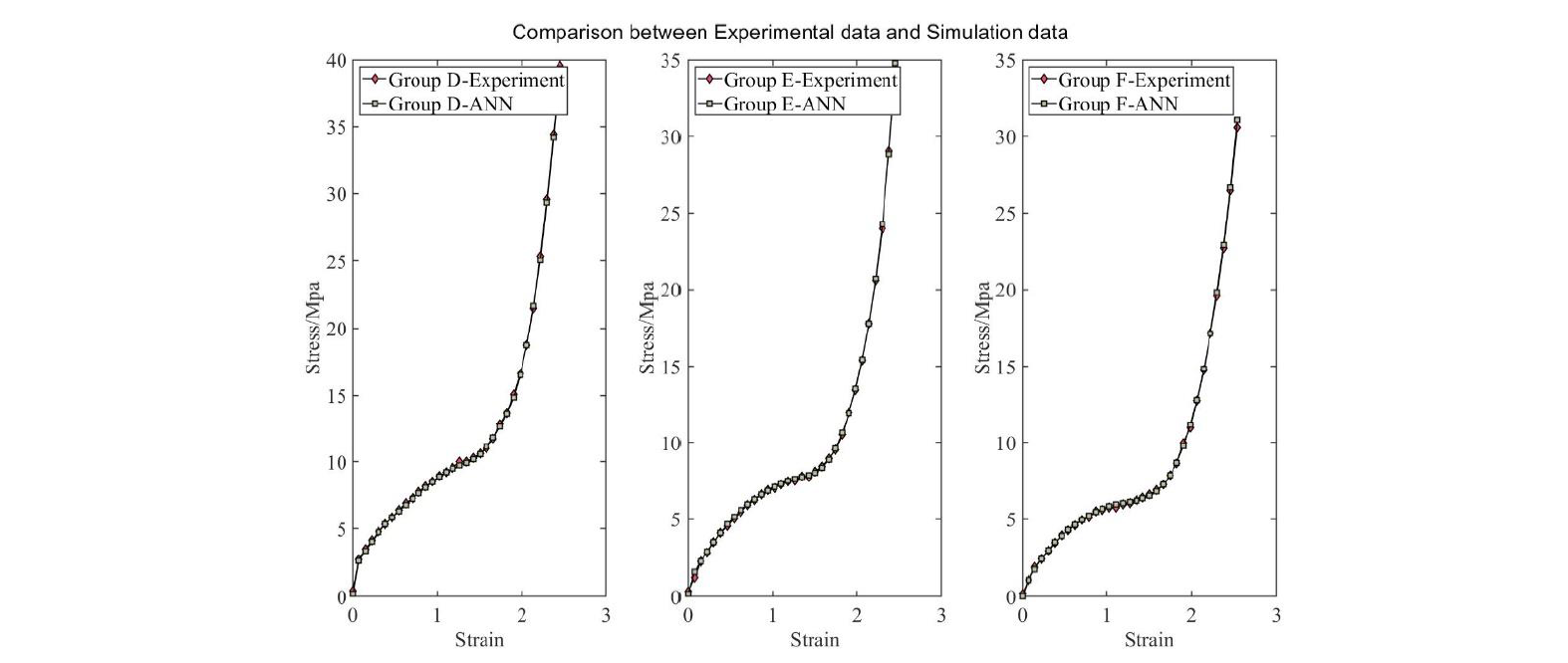
Fig. 7. Comparison between Experimental data and Simulation data in: 1) Group D:90°C,4/s; 2) Group E:95°C,4/s; 3) Group F:100°C, 4/s

Table 4. MSE valve of Group D, Group E, Group F

Comparing with Table 3 and Table 4, with the increase of temperature, the MSE value of different groups are not significantly influenced, which is different to the trend of the various strain rate groups. These groups which have similar level of datasets therefore have similar values of MSE. As a result, in ANN model, this most critical parameter is the number of datasets which will influence the accuracy of the model directly.

The results of 32 s^-1 groups are shown separately in Fig. 8 and Fig. 9. Due to the high speed of the test and the relatively slow rate of the data acquisition system, the number of experimental data points is low (~10), but it can be seen that the stress-strain curve is still captured accurately. According to Fig. 8, the fit is so good that it is difficult to distinguish between experimental curves and simulation results.

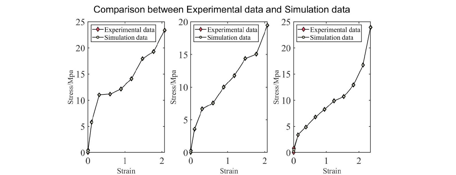
Fig. 8. Comparison between Experimental data and Simulation data for 32s^-1 groups: 1) 90°C; 2)95°C; 3) 100°C

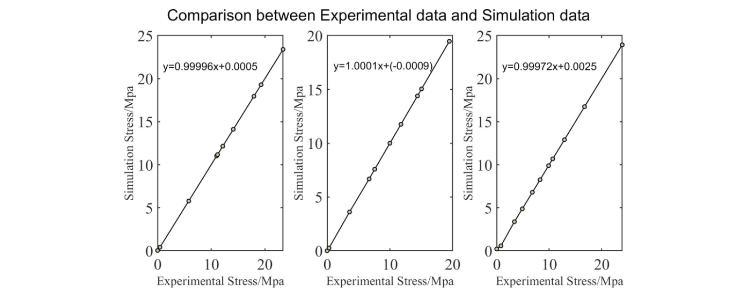
Fig. 9. Comparison between Experimental data and Simulation data for 32s^-1 groups: 1) 90°C; 2)95°C; 3) 100°C

5 Conclusions and future work

A multi-layer feedforward ANN is designed, trained and verified in the current work. Considering the extremely nonlinear behavior of PET’s stress-strain curves, the exhausting searching method is carried to optimize the structure of ANN. This paper has proved that a multi-layer ANN with suitable architecture is able to approximate the relationship between strain and stress under biaxial stretching process for finite deformation of PET at condition relevant to Stretch Blowing Moulding. However the application of ANN for this problem is still at a relatively basic stage. In the future the input variables will be modified to enable the ANN to be structured in such a way that it can be implemented via a VUmat in the commercial software package ABAQUS.