1 Introduction

Additive manufacturing (AM) processes involve the addition of material, typically via the use of a strong heat source used to melt or bond materials together. Those methods are revolutionary in allowing a better freedom of design for the creation of parts. However, the complexity of the process combined with the very high temperature gradients that can arise in the parts can contribute to issues like thermally distorted parts and unwanted residual stresses. The simulation of such processes is thus of great importance for their use in the industry.

Additive manufacturing processes introduce specific challenges for their finite element simulations. Indeed, they often impose a very fine discretization due to the process itself (layers can be as small as a few 𝜇𝑚 in AM). Moreover, they induce a dynamic expansion of the computational domain due to the addition of material.

Thermal and thermo-mechanical simulations of additive manufacturing already exist in the literature [4] [5] [6] [7]. A lot of past AM simulations involve very small deposits or have approximated the process due to the high cost of the simulations. Due to this fact more recent articles have started using advanced numerical methods to allow for less costly simulations, this includes multi-scale approaches [8] and remeshing approaches [9] [10].

The main goal of this work is to implement an efficient part-scale additive manufacturing model in Metafor [1], which is a fully implicit in-house Finite Element code developed at the University of Liège. The first step is to enable material addition in Metafor models. The second step is to decrease the CPU time of the simulations by the use of more sophisticated mesh-management methods. The present work only considers thermal simulations at the time.

Metafor already allows for thermal simulations, the main challenge is to implement a dynamically growing mesh to model the addition of matter in an additive manufacturing process. This dynamically changing mesh induces evolving boundary conditions which need to be dealt with (boundary conditions for such simulations include convection and radiation boundary conditions and a heat flux boundary condition to model the heat input). The solution to handle this dynamically changing mesh is to follow a similar approach as the element-deletion algorithm implemented in Metafor in the scope of crack propagation [2]. This implementation allows the deactivation of finite elements based on certain failure criteria. The present work adapts this method to obtain “activation” criteria.

The second objective of this work is to obtain faster AM simulations by implementing a dynamic remeshing strategy to reduce the computational cost. A choice of remeshing using non-conformal meshes was made, similarly to what is done in the literature in [9]. This type of remeshing generates hanging nodes which are then handled via the use of Lagrange multiplier constraints. The data is then transferred between meshes with a projection method involving finite volumes [3]. The model is compared to a 2D thermal simulation of Direct Energy Deposition (DED) of High-Speed Steels published by Jardin et al. [4] for verification of the results.

2 Description of the problem

A schematic of a basic AM simulation at the part scale can be observed in Fig. 1. The typical boundary conditions to consider are radiation and convection boundary conditions. Those boundary conditions need to adapt as the mesh evolves to continually remain on the boundary of the piece. The heat input of the laser can be modelled by a surface heat flux boundary condition which only needs to be active on the currently activating element (i.e. the element at the laser position). An example of the evolving simulation between two time steps can be seen in Fig. 1. The position of the laser is represented by a “laser tracker” defined as a moving geometrical entity (e.g. green point on Fig. 1). As the laser position is updated to a new position, the mesh is modified accordingly by the activation of the corresponding finite element and all the connecting boundary conditions are updated.

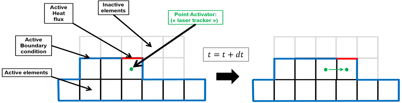
Fig. 1. Example of a basic additive manufacturing simulation, with active (black) and inactive (grey) finite elements, with evolving convection and radiation boundary conditions (blue), with a heat flux boundary condition modelling the heat of the laser (red) and with a “laser tracker” point modelling the current position of the laser (green)

3 Element activation method

An element activation criterion is implemented to allow the dynamic activation of elements throughout the simulation. A geometrical criterion is used. The laser tracker moves with a path mimicking the wanted laser path, the activation criterion then consists in checking which element contains the laser tracker. At each new time-step, the criterion is checked for each element which is then activated accordingly. The boundary conditions are updated as follows: when an element is activated, each adjacent boundary condition is checked to know if it lies on the edge of the activated mesh. If it is on the edge of the mesh, it is considered as a boundary and it is activated. Otherwise, it is not considered as a boundary and the boundary condition is automatically deactivated. A special treatment is given to the heat flux boundary conditions which need to be activated only on the currently activating element, i.e. the element currently containing the “laser tracker”.

A big advantage of this method is its simplicity of use. The user solely has to define the laser tracker and the laser path and both elements and boundary conditions will automatically update according to the given path. One can, of course, imagine a more complex geometrical entity to model the laser to obtain a more complex activation. One could also consider a different activation criterion. An example of a different type of activation criterion is described in [5] for thermo-mechanical simulations where a geometry-based criterion is used for the thermal activation of elements and a temperature-based criterion is used for the mechanical activation of elements.

4 Simulation

This AM model is used to reproduce results from Jardin et al. [4] featuring a 2D thermal simulation of Direct Energy Deposition (DED) of High-Speed Steels. The sample dimension is 40x40mm² with a deposit height of 27.5mm. It is deposited on a 100x100mm^² substrate of 40mm width. The laser power, nozzle scanning speed, powder feed rate, and the pre-heating temperature of the substrate are respectively fixed at 1100W, 6.87mm/s, 76mg/q and 573.15K. The thermal conductivity, density and specific heat capacity were measured for samples extracted from the deposit and the substrate [11]. Radiation and convection boundary conditions are considered in the simulation with a radiation emissivity set to 1 and a convection coefficient set to 230 W/m² K. The laser heat flux was fitted in the 2D model based on the substrate temperature experimentally measured. The simulation is well suited for the verification of our model. Indeed, it is a 2D thermal simulation with known material parameters. Furthermore, the data for the temperature over time of multiple thermocouples are available, both in the substrate to check for global temperature change in the structure, and in the deposit to verify that the simulation gives accurate results close to the activating layer, this zone being the one with the highest temperature gradient (Fig. 2).

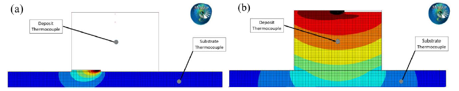
Fig. 2. Reproduction of the simulation from Jardin et al.[4] in Metafor. The points at which the temperature over time is available from Jardin et al. [4] are represented in grey
(a) Beginning of the simulation, (b) Near end of simulation

One can see on Fig. 3a that the temperature curves almost perfectly match for the point inside the deposit, even during the first few seconds of activation. This result shows that the evolution of the mesh and the activation and deactivation of the boundary conditions are correctly implemented over time. The results are also similar for the point in the substrate (Fig. 3b) which shows that the global temperature change in the structure is similar for both simulations. A comparison of the overall temperature fields can also be observed in Fig. 4 with comparable results between the simulations. The Metafor simulation is therefore verified against the simulation from Jardin et al. [4].

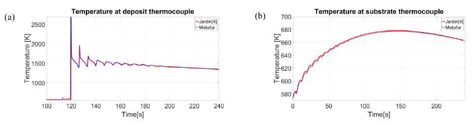
Fig. 3. Temperature at the two thermocouples over time from Jardin et al.[4] (red) and from the Metafor simulation (blue)
(a) Temperature at the substrate thermocouple, (b) Temperature at the deposit thermocouple

Fig. 4. Temperature field in the deposit near the end of the simulation
(a) Jardin et al.[4], (b) Metafor

5 Remeshing

Since the goal of this project is to obtain fast AM simulations, a remeshing method is introduced. Indeed, additive manufacturing simulations often requires the use of extremely small finite elements simply due to the process parameters themselves (the layers added in AM processes can be as small as a few 𝜇𝑚). This creates very costly simulations even for small pieces and the computation cost can even become prohibitive for large parts. Implementing a remeshing method can help overcome this issue by allowing the mesh to be refined only in a zone close to the currently activating layer. The elements in zones far away from the current layer can then be coarsened to decrease simulation cost.

5.1 Remeshing method

The remeshing method implemented in Metafor is straightforward. First, a classical simulation is created. Then, the simulation can be automatically stopped according to a predefined user criterion. When the simulation is stopped, a new mesh is automatically redefined. Finally, the temperature field is transferred from one mesh to the other using projection methods involving finite volumes [3]. This whole process is automatically repeated for each predetermined remeshing trigger without the user’s intervention. The use of this method with strategically chosen remeshing times and zones can significantly reduce the computation time of AM simulations without having a big impact on their accuracy.

An example of a simulation with remeshing in Metafor is schematized in Fig. 5. As stated before, the remeshing can be triggered by a user criterion and it can be done zone by zone. The simulation uses a remeshing trigger defined by a time criterion. Whenever the remeshing is triggered, each zone defined in Fig. 5 can be remeshed independently. In this example one can see that the mesh in zone 1 is remeshed once the simulation starts activating elements in zone 3, the same can be said about the remeshing of zone 2 which is triggered when the elements in zone 4 are being activated.

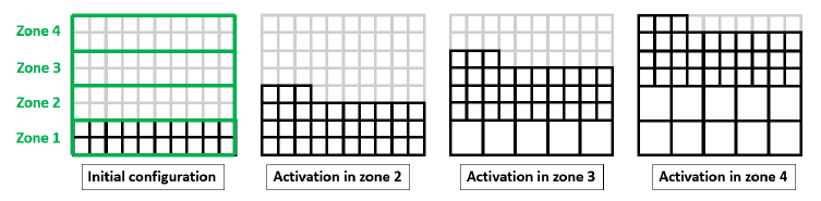
Fig. 5. Example of zone by zone remeshing in Metafor

To allow the remeshing to occur in each zone completely independently of the mesh in the other zones, the created mesh is allowed to be non-conformal between zones. One can see in Fig. 6 that on the boundary of two meshing zones one can thus obtain hanging nodes. Those nodes have to be handled differently because a continuous solution will not be naturally obtained at those locations.

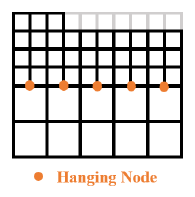
Fig. 6. Example of how hanging nodes are naturally created during the remeshing because we allow zone by zone non-conformal meshes

5.2 Hanging Node

The temperatures at hanging nodes need to maintain continuity in the temperature field. It is thus obvious that their value has to follow (see Fig. 7a):

The chosen method to impose this constraint in Metafor is to use Lagrange multiplier constraints. The basic principle of such constraint is to add a degree of freedom 𝜆 for each hanging node and to add an equation to the system that derives from the minimization of the Lagrange function (𝐿) relative to the constraint we want to impose, in this case:

It follows that if such constraint is added to the FEM system each time a hanging node is created, the solution of the full system will then naturally fulfill the constraint and we will get a continuous solution at the hanging nodes. The method can be extended to mechanical degrees of freedom in the case of thermo-mechanical simulations.

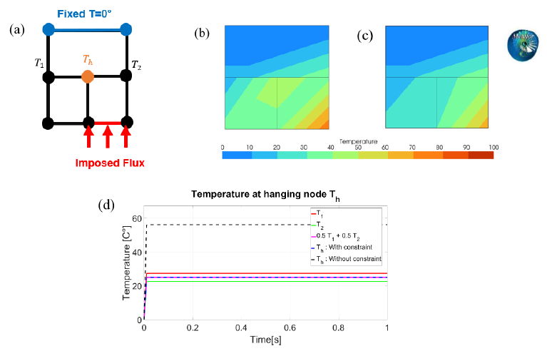
Fig. 7. Simulation showing the correct implementation of hanging nodes in Metafor
(a) Schematic of a simple test case containing one hanging node, (b) and (c) temperature fields respectively without and with a Lagrange multiplier constraint added at the hanging node, (d) temperature over time of the expected value of 0.5𝑇₁+0.5 𝑇₂ and the numerical values obtained with and without the constraint

A simple 2D simulation where a Lagrange multiplier constraint needs to be used to maintain a continuous temperature field is represented in Fig. 7. The thermal simulation has an imposed heat flux on one element and a fixed temperature boundary condition on the other end (Fig. 7a). The obtained temperature at the hanging node can be observed on Fig. 7d, the expected value of 0.5𝑇₁+0.5𝑇₂ is also plotted for comparison, one can check that we indeed obtain 𝑇_ℎ=0.5𝑇₁+0.5𝑇₂ when the constraint is applied to the model. Moreover, the temperature fields without (Fig. 7b) and with (Fig. 7c) the use of a Lagrange multiplier constraint show that the field is discontinuous when no constraint is imposed and is continuous once the constraint is added. This test displays the importance of the particular handling of the hanging nodes and showcases their correct implementation in the code.

5.3 Remeshing simulation

The previous simulation from Jardin et al. [4] is simulated again, this time using remeshing. The remeshing is defined over 18 remeshing zones each containing two layers. The remeshing parameters are chosen such that a remeshing will trigger when the first element of a zone is being activated. The remeshing algorithm will then remesh each zone that is at least 𝑛_𝑟 layers away from the currently activating layer, 𝑛_𝑟 being a user-defined parameter. The actual remeshing operation is defined to halve the number of elements in a zone. A schematic of the simulation can be observed in Fig. 8.

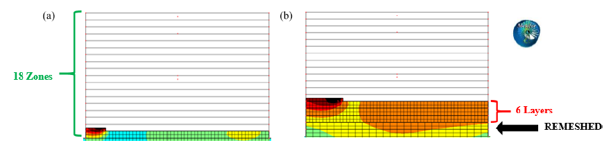
Fig. 8. Metafor simulation with remeshing
(a) Division in 18 zones, (b) Remeshing is triggered at the beginning of each zone, 𝑛𝑟=6 layers below the activating layer

Four simulations are realized with 𝑛_𝑟=[2,4,6,8] (layers) to determine the distance at which the remeshing does not significantly influence the results, the temperature curves are given at the substrate and deposit thermocouple in Fig. 9.

One can see in Fig. 9a and 9b that the temperature curves are similar but the results do not perfectly match. A more thorough investigation was thus realized on the deposit results to observe the influence of the remeshing distance 𝑛_𝑟. The remeshing obtained with 𝑛_𝑟=2 (Fig. 9c) shows the most significant differences with respect to the model without remeshing, one can see differences rising between the two curves almost from the beginning of the simulation, this result is expected since the temperature gradient remains quite high 2 layers away from the activating layer and a refined mesh should thus be used in that region. The simulation obtained with 𝑛_𝑟=4 (Fig. 9d) shows a much better accuracy in the first few peaks, showing that this distance is sufficient to correctly model the activation of the current layer, but there are still significant differences rising later in the simulation which could suggest that the temperature gradient becomes too high at this distance of the activating layer. The remeshings obtained with 𝑛_𝑟=6 (Fig. 9e) and 𝑛_𝑟=8 (Fig. 9f) produce very similar results with only a slight improvement between the two curves, a remeshing distance 𝑛_𝑟=6 thus seems to be sufficient to maintain a good accuracy on the result while remeshing. The most important part of this analysis is that we could determine a certain remeshing distance (here 𝑛_𝑟=6) at which the accuracy of the results was not significantly impacted.

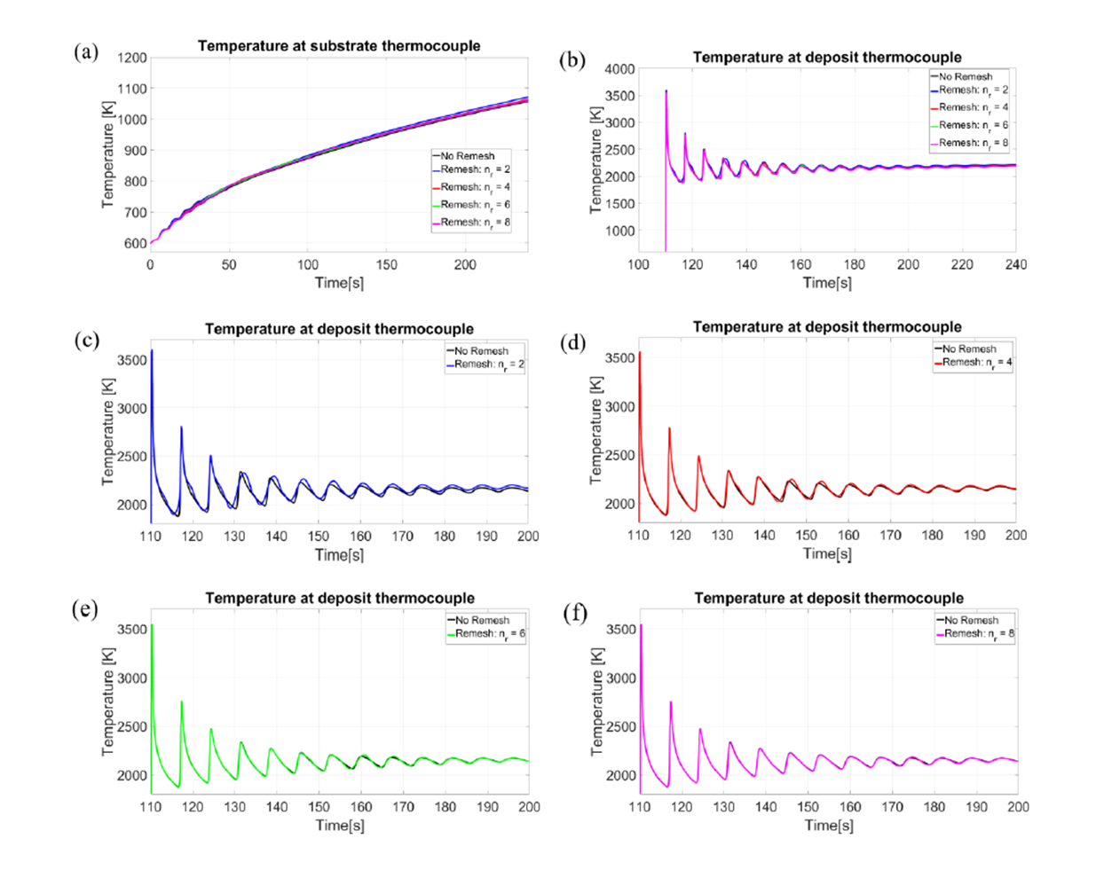
Fig. 9. Metafor results for simulations including remeshing compared to the Metafor simulation without remeshing. The curves are from a simulation without convection and radiation boundary conditions
(a) Temperature of the substrate for all curves, (b) temperature of the deposit for all curves, (c) Zoom on the deposit temperature for 𝑛_𝑟=2, (d) Zoom on the deposit temperature for 𝑛_𝑟=4, (e) Zoom on the deposit temperature for 𝑛_𝑟=6, (f) Zoom on the deposit temperature for 𝑛_𝑟=8

6 Conclusion

This work showed the basic steps required to implement additive manufacturing simulations in an existing FEM code. The impact of a dynamic remeshing strategy using non-conformal meshes was then compared to a classical AM simulation. A good accuracy was obtained on a 2D thermal simulation with a remeshing halving the number of elements during the simulation. However, the remeshing method has multiple drawbacks. Firstly, the simulation is less accurate than with a fully refined mesh, although it has been shown that a good accuracy can be maintained with correctly chosen remeshing parameters. Secondly, the method is computationally costly because the data needs to be fully transferred from one mesh to the other at each remeshing operation, this can mitigate the overall CPU gain of the method. Future developments will thus include an improvement of this data transfer operation which can be made more efficient by implementing methods particularized to this specific type of simulation. The extension to 3D AM simulations without remeshing is already done in Metafor with plans to extend to 3D remeshing simulations as well. Other future developments will include the extension to thermo-mechanical simulations.