1 Introduction

Many additive manufacturing (AM) processes involve melting and solidification. Such processes come with common drawbacks that include thermal distortion after cooling, porosity, unwanted heat treatment or bad surface quality. These issues stem from the extreme complexity of the process combined with a lack of experience. Better simulation methods are needed at all length scales, where we are focusing on the mesoscale, where the evolution of the liquid melt pool, convective flows, heat transfer and phase transition occur. We have chosen to use the so called particle finite element method (PFEM), as it is well suited for these type of simulations for reasons that will be briefly discussed. One particular difficulty lies in the modelling of phase transition and the release or absorption of latent heat. The latent heat term is highly non-liner and thus makes convergence more difficult, making a good mesh resolution at the phase change interface necessary. This article will focus on mesh refinement and convergence in PFEM when phase change occurs.

2 Methodology

2.1 The particle finite element method

The particle finite element method (PFEM) is a hybrid method combining the flexibility of a Lagrangian particle method with the robustness of a classical finite element method (FEM) formulation [1]. It has been recently introduced to treat free-surface fluid flow problems, including polymer melt flows [2] or nuclear melt-downs [3] and fluid-structure interaction [4], but also applications such as metal forming [5] and ground excavation [6]. The ability to treat solids and fluids alike and the natural representation of free-surface deformation make the PFEM ideal to simulate additive manufacturing at the mesoscale.

Because the PFEM is a Lagrangian method, the material is fully represented by particles at which the solution (position, velocity, pressure, temperature etc.) is stored. The key concept is the automatic generation of a new computational mesh at each time step. Such a temporary mesh is then used to solve the equations using classic large deformation FEM at a given time step. Once the particles have moved, a new mesh is generated from the cloud of particle points (usually using a Delaunay triangulation), thus avoiding an otherwise unacceptable distortion of the mesh.

Using only a simple mesh generation algorithm such as a Delaunay triangulation, one will always obtain a convex shape around the cloud of particles (Fig. 1 a → b). In most cases this is not desired, as the volume of the modelled material may have some locally concave surface (e.g. valleys of surface waves, compressed surface of deflected beam). In other cases we may even have the volume of the material splitting up into smaller volumes, such as splashing in fluids, or fragmentation in solids. The remeshing fills the empty space with elements regardless. These elements are generally larger and significantly skewed, sometimes even slithers. The alpha shape algorithm [7] offers a simple criterion to detect these elements that occupy the empty space. Once detected (Fig. 1 c), they can be deleted, leaving behind only the elements that occupy the actual volume of material (Fig. 1 d). The material’s boundary is implied by the edge of the remaining mesh. This means that when the material deforms under an external load, the boundaries of the material are automatically captured, without the need for an explicit interface tracking method.

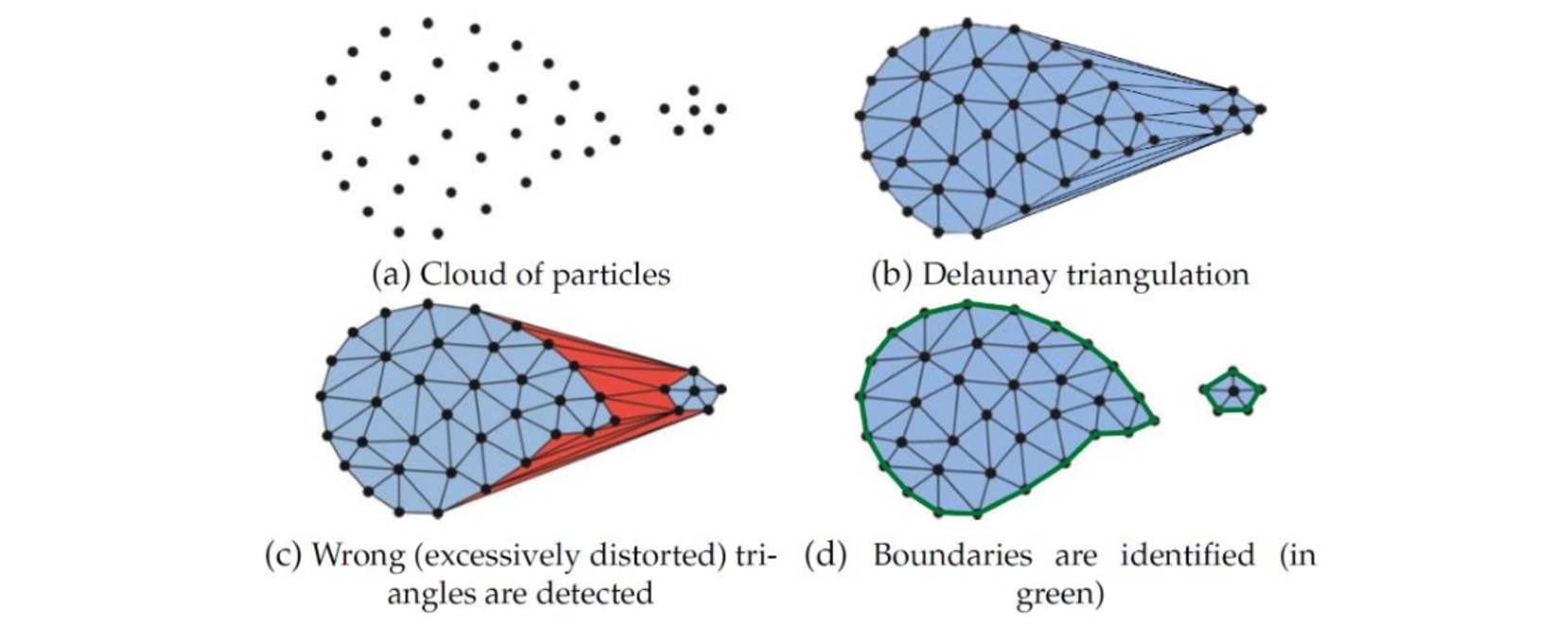
Fig. 1. Schematic of a remeshing step in PFEM. Taken from Cerquaglia [8].

The presented implementation of the PFEM is only 2D, where the mesh consists of linear triangles. Integration at the element level is done using Gauss quadrature with only one integration point.

2.2 Governing equations

To simulate additive manufacturing at the meso scale, a thermo-fluid and a thermo-solid and the transition from one to the other need to be modelled. We use the conservation of mass, momentum and heat for each. The heat equation (1)

where 𝜌 is the density, c_p is the specific heat capacity at constant pressure, T is the temperature, k is the conductivity, Q̇_l is the heat source, and S_L is the absorption or release of latent heat upon phase transition is combined with the well-known Navier-Stokes equations (NSE). All the equations are used throughout the solid and liquid regions. For the case discussed below, even all the material properties are kept constant in all regions. Since the NSE are for Newtonian fluids, we use an extra source term that adds a very high flow resistance, when the fluid falls below the melting point T_m. This holds the solidified particles in place and prevents further deformation. The source term is based on the Carman-Kozeny equation, which is normally used for porous media, but also a common way to use a fluid dynamics code for solidification in the context of AM [9].

Next, we define the liquid fraction f_l as a function of the temperature:

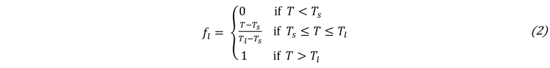
where T_s is the solidus and T_l the liquidus temperature. In the case of isothermal phase change (as in our case) T_s=T_l=T_m, with Tm being the melting temperature. Note that in this case, the liquid fraction is described by a step function.

The liquid fraction is used by the latent heat term S_L in the heat equation (1):

where L_m is the specific latent heat of melting of the material. When the phase does not change, the derivative of the liquid fraction remains zero. However, when the liquid fraction changes over time, i.e. at transition, the term S_L is non-zero. Since L_m is very large in magnitude, while df_l/dt can also become very large, this term is dominant during phase transition. Furthermore, this term is nonlinear, as f_l is not a linear function of T. Both aspects represent a major challenge from the numerical point of view.

Apart from that, it is noteworthy that, since PFEM uses linear shape functions for pressure and velocity, the Ladyzhenskaya– Babuška–Brezzi (LBB) stability criterion is violated. The so called Pressure-Stabilizing Petrov-Galerkin (PSPG) formulation is thus used to stabilize the solution [8]. All equations are integrated in time using the backward Euler scheme, which is fully implicit and first order accurate.

2.3 Solution strategy

The NSE are solved in a monolithic approach, while the heat equation is staggered. The heat equation is solved first at each time step to update the temperature field, then the NSE are solved using the updated temperature field to obtain the pressure and velocity fields. The resulting velocity field is then used to update the position of each particle at the next time step, where the new position of all particles is used to generate a new mesh, as explained above. A Picard iteration is used to solve the NSE. On the other hand, to ensure a robust and efficient convergence of the solution despite the strong non-linearity of the heat equation, this latter equation is solved using a Newton-Raphson algorithm. Additionally, a line search algorithm and a regularization of the latent heat term are performed, as proposed by Celentano et al. [10].

3 Mesh refinement

To further increase efficiency and accuracy, the mesh is locally refined in regions with large gradients of velocity or Temperature. While mesh refinement / adaptation is a well-known and proved technique, its application in the context of the PFEM is less straightforward. Mesh adaptation involves three main elements: the definition of the target mesh size, the addition/deletion of nodes according to this target value, and the adaptation of the alpha-shape technique to eliminate unwanted elements.

3.1 Mesh refinement in the particle finite element method

To refine a mesh in the PFEM, particles are added to locally increase the density of particles. A higher density of particles will result in a finer mesh produced by the Delaunay triangulation. In the present case, particles can be added to the centroid of a triangle or an edge, splitting them in smaller elements. Because the solution is stored at the nodes, the new particle must be initialized with the interpolated value of the solution of the other particles belonging to the element that is refined. Since the PFEM traditionally uses linear shape functions, this interpolation results in no loss of information. On the other hand, removing a particle to coarsen the mesh introduces an error, because the solution stored at this particle is lost. This may result in an artificially increased diffusion of momentum and heat. If the coarsening only occurs in regions where the gradients of velocity or temperature are not changing significantly, the error is negligible, but this is generally not the case, as refinement and coarsening take place in the regions of high gradients.

3.2 Choosing the target mesh size to converge with latent heat

The latent heat that is released or absorbed upon phase transition is a source term that can be highly non-linear. The element size around the phase change front must be small to capture the exact location and to achieve convergence. First a simple calculation to estimate the required element size is performed. Isothermal phase change is assumed, as it signifies the worst case scenario.

Since elements have only one Gauss point to integrate the latent heat term (eq. 3), which contains a step function from the liquid fraction (eq. 2), any given element can fully transition from solid to liquid or conversely in a single time step. This means that the term df_l/dt≈Δ𝑓_l/Δ𝑡=±1/Δ𝑡, where Δ𝑡 is the chosen time step. Together with the known constants, the source term maximum value S_Lmax can be determined. The integration of this term over an element k with one Gauss point is

where A is the element’s area and w is the weight of the Gauss point, which is 1 in this case. As a guideline, equation (8) can be solved for 𝐴 to get the required element size, if we assume that this source term should have a similar magnitude as other terms in the heat equation. Having an estimate for the required element size at the phase change front, finding the regions that need refinement is described in the following section.

3.3 Refinement strategy

If the mesh refinement is supposed to be dependent on the appearance of the latent heat source term, a function that controls the refinement must be defined. The input is the temperature and the output is the desired element size, which we call characteristic element length L_c. It refers to the edge length of an equilateral triangle of area A. A piecewise linear function is defined, so that the fine mesh is within an interval of T_m-1/2ΔT_fine < T < T_m+1/2ΔT_fine , where ΔT_fine is a user defined tolerance. We use ΔT_fine=10 K. Outside of this interval, the mesh can be coarse. To avoid an excessively abrupt change between fine and coarse mesh, a transition region is possible using some interpolation.

Note that it is important to perform the coarsening of a refined region gradually. Particles are checked in a random order and if they are in a too dense region, they are removed. Preforming this checking and deleting in a random order has the side effect of producing a patchy mesh, where some patches are denser than others. When coarsening in several steps, the dense patches will be automatically targeted first in each new step, actively reducing the patchiness and producing better quality elements.

If the solution changes rapidly from one time step to the next, the solution-based mesh refinement may be lagging behind, since the mesh is defined using the last converged solution of the previous time step. In such cases, the refinement and remeshing can also take place in the middle of a time step, i.e. after a few iterations. Then the mesh refinement is based on the current solution, even if the solution is not fully converged yet.

4 Example test case

In order to assess the impact of mesh refinement around a transition front the 1D isothermal phase change in a semi-infinite slab is investigated. The test case is taken from Celentano et al. [10], who compare their own simulation with an analytical solution [11]. They use a more advanced technique to capture the exact location of the phase transition front, even when it runs across an element, by splitting the element in two subdomains, where the spatial integration becomes accurate. The present approach is not able to do this, so less accuracy and more difficulties converging are expected.

4.1 Simulation setup

An elongate rectangle with an initial temperature T₀ above the melting point T_m is given, with all walls adiabatic, except the left wall. There, a constant low temperature is imposed to gradually freeze the entire domain from left to right.

Fig. 2. Schematic of semi-finite slab test by Celentano et al. [10].

Fig. 2 shows the schematic simulation setup, with all the relevant material properties. Note that there is no mechanical force acting, so not deformation takes place. Since the case is 1D, the height of the domain does not play a role and is chosen to be 0.5 m.

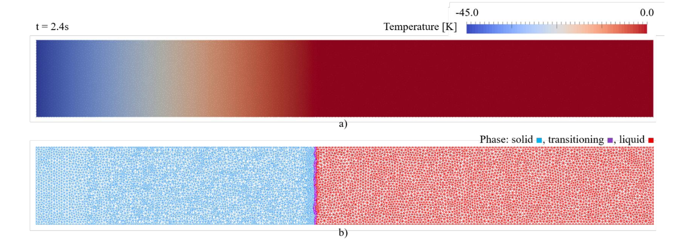
Fig. 3. Temperature field a) and phase field b) after 2.4s. The refined mesh following the transition region (purple), while solid (blue) and liquid (red) are mostly coarse.

Fig. 3 shows the resulting temperature field a) and phase field b) at an arbitrary point in time. The transition region is not a razor sharp and straight line for two reasons: firstly, any element can only be fully liquid or fully solid, due to the single Gauss point per element. The phase change front would be a line that would zig-zag along the edges of the randomly oriented elements. A straight line is not possible with an unstructured rigid mesh. Secondly, the regularization is active in a small interval around melting temperature (±0.01 K). Highlighting this region gives a better idea of where the latent heat term becomes non-zero, since this is the region where the fine mesh is required.

4.2 Results and discussion

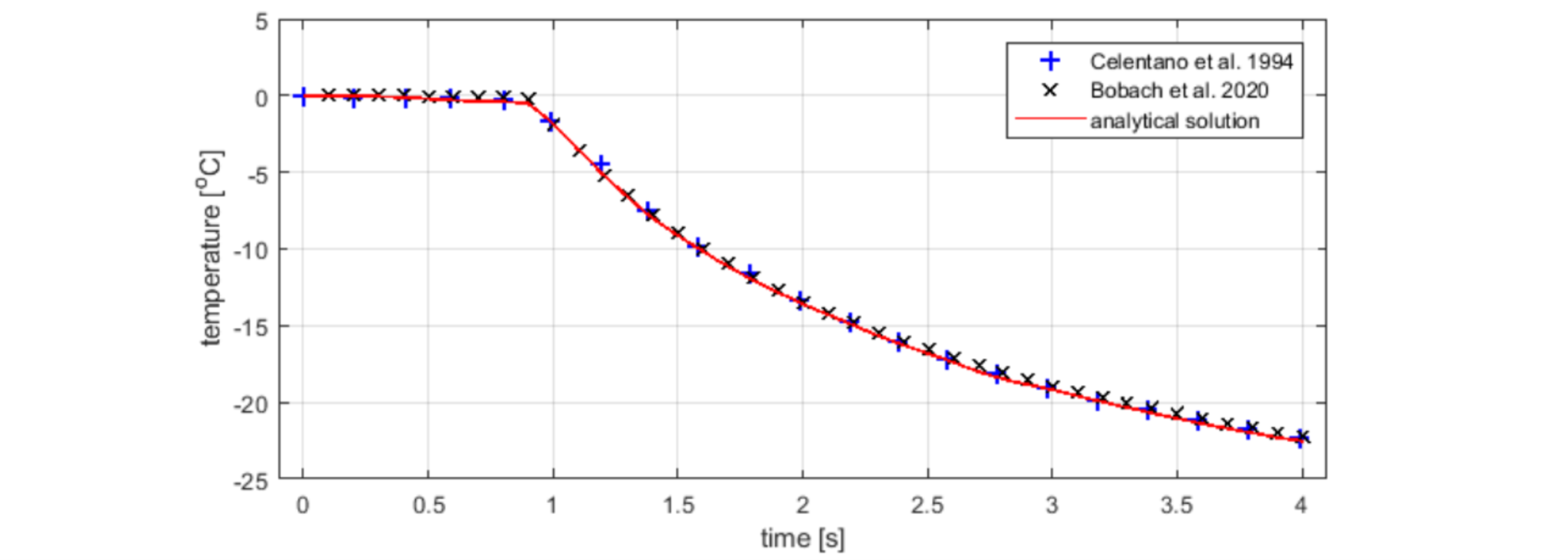
Fig. 4. Comparison of temperature over time at 1m distance from the left boundary. A smaller time step in chosen by us (0.1 s) instead of 0.2 in the original work of Celentano et al. [10].

The reference by Celentano et al. [10] includes an analytical solution [11] to the temperature at 1m distance from the left boundary. Comparing their simulation results and ours in Fig. 4, we find that there is a good agreement between the different approaches. A slight deviation of our results (black crosses) is observed just before the phase change front passes the 1m mark (the kink in the curve) and towards the end of the observed time interval. Both times, the temperature is slightly higher. The difference could be due to the different time step or the different mesh used, since ours is a non-uniform, irregular mesh, while Celentano use a much coarser Cartesian mesh. Their use of the improved spatial integration method also shows excellent accuracy, as expected, while our mesh refinement is more of a brute force technique. Given the much simpler implementation of the remeshing presented, it can serve as a viable first step when encountering the highly non-linear latent heat term.

5 Future outlook

Despite the cost savings of an adaptive mesh, further improvement can be made by implementing the integration method described by Celentano et al. [10]. This method is even faster, since it can use an entirely coarse mesh, without any refinement. The extra cost of the more complex implementation of the method itself, however, is negligible. Furthermore, as mentioned above, a possible improvement of the accuracy could also be achieved with their method.

Other than that, there are many more steps that need to be taken before our code can run AM simulation cases. Most importantly, the shift from 2D to 3D is necessary. Also, many of the physics required for such simulation are already implemented, but not shown in this paper (e.g. surface tension and Marangoni effect, buoyancy, temperature dependent material properties, simple laser heat sources), while other are still missing (elasto-plastic solid, powder, more advanced laser heat sources).

6 Acknowledgements

The authors are grateful for the funding provided by the Fonds de la Recherche Scientifique-FNRS trough a Fria scholarship.