1 Introduction

Nowadays, wire-arc welding-based additive manufacturing (WAAM) is an attractive alternative for the production of near-net-shape parts with complex geometry. With this technology, the required shape is built layer-by-layer by a deposition of a consumable welding wire, where the welding arc is a source of heat. Because the process itself involves thermo-mechanically complex phenomena, Finite Element-based virtual models are commonly employed to optimize the process parameters [1]. The finite elements (FEs) activation is applied in numerical investigations of deposition of a welding wire, where the melting temperature is employed as the activation criterion [2]. There are two procedures available for dealing with inactivating FEs in the FE numerical model [3]. The first procedure is based on assigning special thermo-mechanical material properties to inactivate FEs to achieve that these FEs do not affect the already activated FEs. Taking into account this procedure, the number of FEs and the unknowns in the numerical model is the same during the computation time. The second procedure is based on the inclusion of the FEs into the numerical model when the FEs activation criterion is fulfilled. The number of FEs and the unknowns in this procedure increases during the computation, so the computation effort is smaller. Heat source due to the welding arc, which heats the FE domain being activated in the next time step, is usually considered as Goldak double ellipsoidal heat source [4]. The geometry of the weld cross-section is usually simplified [5], but the geometry of the weld cross-section in the numerical model influences on the part thermo-mechanical state during and after the welding process. To obtain a realistic mechanical state, like residual stress and distortion, of the part [6], it is important to compute the temporal distribution of the temperature field, taking into account realistic boundary conditions.

This paper presents advanced computational modelling of the WAAM of a tube. A thermo-mechanical numerical model of the process is calibrated against experimental data, measured as temperature variation at the acquisition point. The virtual modelling starts with a preparation of the part geometry in CAD software. The geometry of the single-layer cross-section is assumed close to real weld cross-section. The geometry is then exported to a G-code format data file and used to control a three-axis CNC machine. On the other side, the same code serves as an input to in-house developed code for automatic FEs activation in a material layer-adding process FE computer simulation. The time of activation of the FEs is directly related to the material deposition rate. The activation of the FEs is followed by a heat source, described by a Goldak double ellipsoidal power density distribution [4]. The thermo-mechanical problem is solved as uncoupled to speed-up the computation.

2 Computational Modelling of WAAM

A proposed computational model of WAAM process is described by the flowchart, presented in Fig. 1.

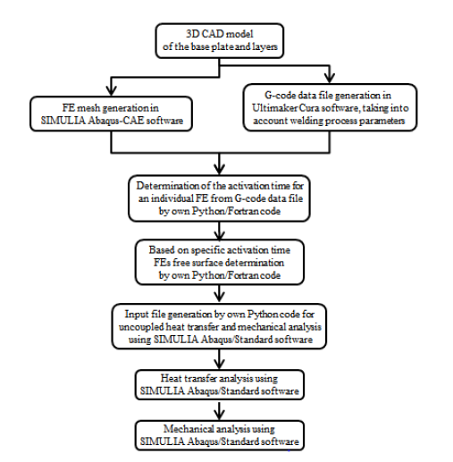
Fig. 1. Flowchart of computational modeling of the WAAM process

The initial step in this procedure is the preparation of the 3D CAD model of the base plate and layers geometry (see Fig.2). The geometry of single-layer cross-section should be as close as possible to the expected real weld cross-section.

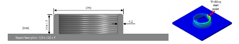
Fig. 2. A part geometry composed from the square base plate and 10 welded layers

This step is followed by two steps, FE mesh and G-code data file generation, which could be processed in parallel. FE mesh generation is done with SIMULIA Abaqus-CAE software [7]. In preparation of the G-code data file by Ultimaker Cura software [8], welding process parameters, like deposition speed, should be taken into account. This G-code data file is later used for CNC machine control in the actual welding process. Based on the generated FE mesh data and the G-code data file the determination of the activation time for an individual FE is done using our own Python/Fortran code. Knowing the activation time for an individual FE, a time change of free surface used for heat transfer boundary definition in heat transfer analysis is determined by our own Python/Fortran code. Using the Python code, the next step is the generation of two input files for uncoupled heat transfer and mechanical analysis for SIMULIA Abaqus/Standard software. During computation, the FEs are activated in two ways. On one hand, before the start of new layer deposition, FEs of this layer are included in the numerical model. On the other hand, during layer deposition, FEs are activated by changing material properties. By this procedure, the number of FEs and unknowns increases in the numerical model layer by layer, which speeds-up the computation. The thermo-mechanical problem was solved as uncoupled: first the heat transfer analysis and then the mechanical analysis.

3 Experimental Case Study

Welding layer by layer of the circular-shaped sample was done using a three-axis CNC machine (Fig. 3). The machine has a work table that moves in three axes (x: 165 mm, y: 180 mm, z: 220 mm) under the fixed deposition torch. The machine is equipped with a protective box that protects the environment and the machine from UV radiation and spattering during deposition. The work table is electrically isolated from the rest of the system. A Daihen Welbee P500L power source was used for testing. The system is equipped with LinuxCNC motion controller, which enables the synchronous control of all the equipment. The G-code was prepared in the Ultimaker Cura software [8], based on a 3D CAD model. A low spatter welding protocol was used at the welding power source. WAAM was done using 65 A welding current, 14.8 V welding voltage and 240 mm/min welding speed. A mixture of shielding gasses Ar + 18 % CO2 was used at deposition, with a flow rate of 12 l/min. The deposition started at the same location on the circle for each layer. Between each layer, a 30 s pause for cooling of the layer was used. During the deposition, the temperature of each layer was measured using a K-type thermocouple, National Instruments (NI) CDAQ 9174, temperature measuring card NI 9213 and Labview software on a second control computer. Location of temperature measuring is 20 mm along the circle, on the deposited material, from the welding start point, always at the top layer.

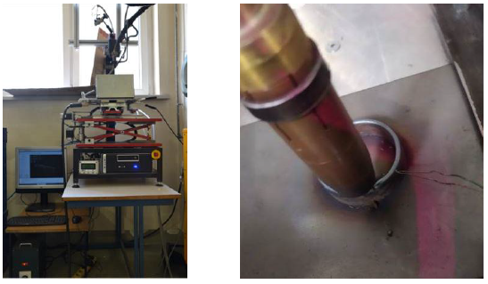
Fig. 3. Experimental welding performed by a three-axis CNC machine

The square base plate has dimensions 120 x 120 x 5 mm (Fig. 2), while the diameter of the welding wire is 1.2 mm. Welding layer width and height are 4.2 mm and 1.5 mm (Fig. 2). In the experiment, 10 layers were performed. The material of the base plate is S235, while the material of welding wire is G3Si1. Chemical compositions of both materials are given in Table 1.

Table 1. Chemical composition of G3Si1 (EN 440) filler wire and S235 (EN 10025) base plate

	C	Si	Mn	P	S	Fe
G3Si1	0.08 %	0.90 %	1.50 %	< 0.025 %	< 0.025 %	Balance
S235	< 0.22 %	< 1.60 %	< 1.60 %	< 0.050 %	< 0.050 %	Balance

4 Numerical Case Study

A 3D numerical model, based on the Finite Element Method, is developed in SIMULIA Abaqus-CAE software environment, taking into account the same geometry as in the experimental case study (Fig. 2). The base plate is meshed with 32.000 3D hexahedral 8 nodes FEs, where the FE mesh refinement is considered in the domain close to the layer deposition area, as shown in Fig 4, left. Each welding layer is structured meshed along the welding path with 15.000 FEs (same FE type as in the base plate), having the same FE topology in the layer cross-section (Fig. 4, right). In the layer cross-section, FE mesh refinement is considered in the domain, which will be after activation in contact with already activated FEs. This is important because in this domain great temperature gradients are expected after FEs activation, where the temperature of the new activated FEs is equal to the melting point. The characteristic length of the FE (1.7 mm) in circular direction is computed from welding speed (240 mm/min) and time increment of FEs activation (0.4 s), so each layer is composed of by 94 FEs activation steps. The time step upper limit in numerical computation is 0.04 s for heat transfer and mechanical analysis. In the computer simulation, the duration of each layer deposition is 37 s, followed by 30 s cooling break. After the 10^th layer, the part is cooled to steady-state.

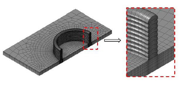
Fig. 4. FE model with the mesh – base plate 32.000 FEs, each layer 15.000 FEs

Temperature-dependent physical properties of welding wire (G3Si1), used in numerical computation, are taken from [2] because of the similarity in the chemical composition of G3Si1 and G4Si1 material, used in [2]. Same properties were used for the base plate. The values considered are presented in Table 2 and Table 3.

Table 2. Temperature-dependent yield stress used in computer simulation [2]

Table 3. Temperature-dependent material properties used in computer simulation [2]

The initial temperature of the base plate is 25°C, while the temperature at FEs activation is equal to meting point, i.e. 1500°C. Boundary conditions in heat transfer analysis on the free surfaces were natural convection and radiation, where the ambient temperature, the film coefficient and the emissivity were 30°C, 20 W/(m² K) and 1.0, respectively. Heat flux in the contact between the base plate and the support table is defined by the support table temperature of 25°C and heat transfer coefficient of 50 W/(m² K). In front of the last activated FEs the heat source following the Goldak double ellipsoidal heat source [4] is considered, where the length and width of the heat source influenced domain is 4.2 mm and depth is 1.5 mm. Speed of the heat source movement is the same as the welding speed.

In the mechanical analysis the base plate is clamped in two opposite sides, where the welding start point is close to one side (see Fig. 2). Computed time evolution of the temperature in the heat transfer analysis is taken into account as a load of the base plate and emerging layers. Because the computed temperature gradient after FEs activation is too big compared to the real temperature gradient in the continuous welding process, computed temporal distribution of the temperature is smoothed at the time of the FEs activation in a way that temperature is averaged over temperature one time step before (t_act -0.04s) and one time step after activation (t_act +0.04 s) and used as a temperature at activation time (t_act).

5 Numerical and Experimental Results Presentation

To verify the presented numerical model of WAAM process, comparison between the computed and measured temperature at the point 20 mm from the start of the layer is performed. In Fig. 5, computed and measured temperature profiles for four layers (1^st, 4^th, 7^th and 10^th layer) are shown, where the solid lines represent computed and solid lines with circles measured temperatures. It is evident that during the welding time interval (0-37 s), the difference between computed and measured temperature is larger than during a cooling break interval (37-67s). A sudden drop in temperature is observed as well at the end of welding time, which happens without a thermal reason. Effect of heating up at the measuring point, which is 20 mm from the start-end point of welding, in initial 10 s after the complete layer is made, and then slow temperature decrease in remaining 20 s is in both cases very similar. Comparing temperatures at the time of the start of a new layer deposition shows a very good correlation between computed and measured temperatures.

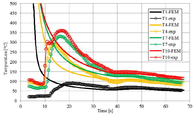
Fig. 5. Comparison of computed (FEM) and measured (exp) temperature at the point 20 mm from the start of the layer for 1^st, 4^th, 7^th and 10^th layer

From Fig. 6 we conclude that the temperature decrease from the melting point is extremely fast due to the large variations between the surface temperature and the melting point at FEs activation in the numerical model. This temperature gradient is larger in numerical computation than in the actual case due to step-by-step FEs activation, where melt material continuous coming in the contact with the warmer surface. This is the reason why in the mechanical analysis computed time evolution of temperature is smoothed.

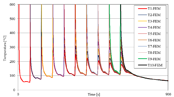
Fig. 6. Computed temperature evolution at the point 20 mm from the start of the layer

The mechanical analysis, based on the FEM, of the wire-arc welding-based additive process, is important due to obtaining insight into the temporal variation of stress-strain state of the part during the process of welding, and the final state after cooling it down to the room temperature and removal of the base plate.

In Fig. 7, radial displacement field on the part after cooling down to room temperature is shown before (a) and after (b) the base plate removal. Due to a decrease in temperature of each layer from the melting point to the room temperature and the consequent thermal contraction, the diameter of the circular-shaped domain of the part decreases. The colder base plate limits the thermal contraction of layers close to it. After its removal, the final dimension of the circular-shaped domain is obtained. The maximal computed reduction of the outside diameter is 0.34 mm, which is 0.65 % of the initial outside diameter of the layer.

For the subsequent mechanical treatment of the part produced this way, it is important to know the level of residual stresses in the domain of the part. In our case, the hoop stresses in the circular direction, shown in Fig. 8 after completing the 10^th layer (a), before (b) and after (c) the base plate removal, are monitored as they can be the reason for vertical cracks in the part if they are tensile. In layers close to the base plate, the hoop stresses during the process of adding layers are tensile in the outside domain, while in the inner domain, they are compressive (Fig. 8a). After cooling the part down to the room temperature, the tensile hoop stresses increase (Fig. 8b), but after the base plate removal, they decrease (Fig. 8c), where the maximal tensile hoop stress is 95 MPa. From cross-section distribution of the hoop stresses, shown in Fig. 8c, the difference between left and the right side is evident. The reason for such difference is that the right cross-section belongs to the start of welding, while the left cross-section is on the opposite side.

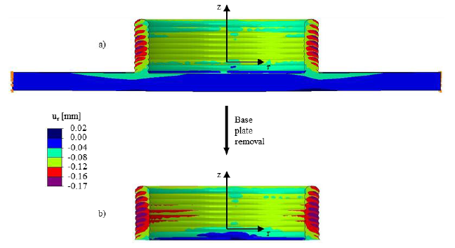
Fig. 7. Computed radial displacement before (a) and after (b) the base plate removal at room temperature

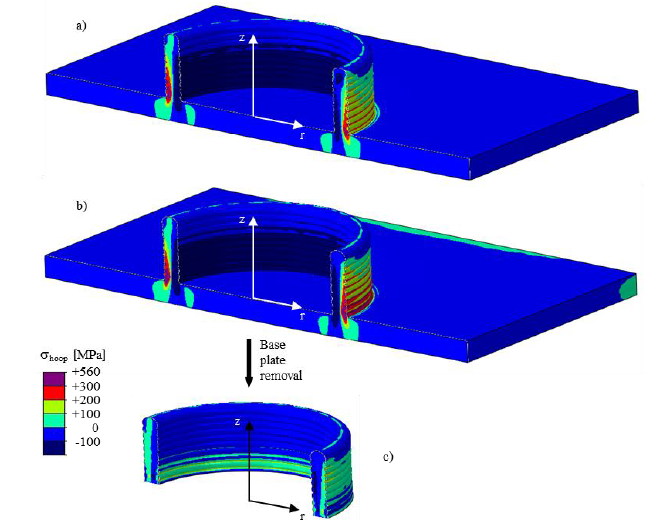
Fig. 8. Computed hoop stress after completing the 10^th layer (a), and before (b) and after (c) the base plate removal at room temperature

6 Conclusion

Advanced computational modelling of the WAAM is presented for the case of the welded part composed from the base plate and 10 welded layers. Modelling starts with a preparation of the part geometry in CAD software, where the geometry of the single-layer cross-section is assumed close to real weld cross-section. The G-code format data file is then prepared based on the obtained geometry and used in our code for automatic FEs activation in the FE computer simulation. The sequential thermo-mechanical analysis of the welding process is performed. Temporal distribution of the temperature during the process and the mechanical state in the part after cooling to the room temperature and the base plate removal, obtained by described numerical procedure, are presented and commented.

Acknowledgements

The authors acknowledge the funding from the Slovenian Research Agency (research core funding No. P2-0263).