1 Introduction

Additive Manufacturing (AM) technology is a unique capability for building complex three-dimensional (3D) objects from computer-aided design models. Among many technologies used for metallic AM, Directed Energy Deposition (DED) is an interesting process that is flexible and adapted to repair operation. This method involves the deposition of metallic powder, which is melted via a focused heat source. DED is becoming widely used in industries such as aerospace [1], bio-design [2].

In order to identify optimal process parameters of AM, a design of experiments is often used [3]. However, performing the experiments of AM to find the optimal parameters is very expensive and time-consuming. The numerical approach, such as the Finite Element Method (FEM), is often employed to simulate the AM process [4]. However, the computing cost of these models remains excessively expensive when performing a large number of simulations. Therefore, it is not suitable to directly conduct uncertainty quantification and optimization of process parameters using these models to achieve a robust solution. To overcome this challenge, Machine Learning (ML) techniques are employed to construct surrogate models representing the complex relations between the process parameter and the temperature history defining the part quality [5]. Thanks to the predictive ML-based surrogate models, the simulations can be performed with a negligible computational cost. Recently, the application of ML to the AM field received significant attention from both the industrial and academic sectors [6, 7, 8]. A comprehensive review of this application can be found in [5].

In AM process, many physical phenomena occur at a short period of time and at a temperature above the melting point of materials. These temperature profiles strongly affect material properties related to the generated microstructures. Some previous studies were performed to develop the ML-based surrogate model to predict the temperature evolution of the AM process. For instance, the Recurrent Neural Network (RNN) was developed to compute the temperature field for an arbitrary geometry with different scanning strategies 6]. Similarly, the temperature field is also predicted by the surrogate model with Bayesian loss function [7]. In addition, in [8], the temperature field was predicted directly by the Physics-Informed Neural Networks (PINNs) without numerical data.

The above ML-based models [7-9] are somewhat complicated (RNN, Bayesian) and only applicable for a few layers. Thus, it is essential to develop a simple ML-based model to directly predict the temperature field of the AM processes with a large number of layers. Based on this review, this study aims to develop a simple ML-based surrogate model to predict the temperature evolution as well as the melting pool size of a DED process of a cubic part with 36 layers. In this article, the data used to train the ML-based model are first generated using the Finite Element (FE) model, which has been validated with experimental data (see Section 2). In Section 3, the ML-based surrogate model is described with its results to predict the temperature evolution and melting pool size during the AM process.

2 ML-based surrogate model for the DED process

In this section, we describe the predictive ML-based model called also the surrogate model to predict the temperature evolution of the DED process. It is built using the following two-step process:

(i) Data collection and data pre-processing,

(ii) Evaluation of the surrogate model parameters.

For step (i), it is very important that the training data is physically representative. Note that this study focuses on bulk experiments of the M4 high-speed steel material powder. The material properties can be found in detail in [9]. Hereafter, the training data is generated by thermal simulations performed with the updated Lagrangian FE code “Lagamine” developed by ArGEnCo Department of the University of Liège [4], Belgium. The convection and radiation boundary conditions are applied as well as the birth element technique to model the process. The classical conduction non-linear equation is reminded as

where T, k, Q_int, cp, 𝜌 and t are the transient temperature, thermal conductivity, the power generated per volume in the workpiece, apparent heat capacity, density and time, respectively. Fig. 1 plots and compares the temperature evolutions at one thermocouple located in the substrate obtained within the experiment and by the 2D FE simulation. The detailed description as well as the schematic of the DED experiment can be find in [4]. As shown in Fig. 1, the result of the 2D FE simulation (representative of the middle track of each layer) is in good agreement with the experimental bulk result. Consequently, the FE model is able to provide high-quality structure data to the ML-based surrogate models described hereafter.

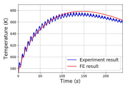Fig. 1: The temperature evolution at one thermocouple of the experimental and FE model.

The dataset used in this study consists in five groups of data. Each group is the data obtained from one FE simulation with a value of input energy Q_int (see Eqn. 1). The five values of Q_int are chosen as 0.8 Q₀, 0.9 Q₀, 1.0 Q₀, 1.1 Q₀, 1.2 Q₀, in which Q₀ = Q_reference = 1 W/m³. The data group obtained from Qint = 1.0 Q₀ is used for further validation and the remaining four data groups are used for training.

Each data group contains 4.8 million data points (see details below). Consequently, a total of 19.9 million data points is used for the training of the FFNN-based model. For step (ii), a FFNN is chosen as it has advantages in approximating highly non-linear and high-dimensional functions. However, training the FFNN with such a small dataset might lead to the over-fitting problem. As a consequence, the training dataset is partitioned into a training dataset and a validation dataset. Beside the input energy, nodal coordinates and time, five additional features are considered as input features to boost the performance of the FFNN-based model including the laser head location in x- and y-direction, the distance from each sampling point to the laser head in x- and y-direction and the current printing layer at each time-step. Note that these additional features are also used in the work of Fetni et. al [11]. For any point of interest, the following 9 features are defined (see Fig. 2).

(i) The input energy (Qint)

(ii) x-nodal coordinate (xp)

(iii) y-nodal coordinate (yp)

(iv) Time

(v) The laser head position at x-coordinate (xl)

(vi) The laser head position at y-coordinate (yl)

(vii) The distance from laser head to each sampling point in x-direction (dx)

(viii) The distance from laser head to each sampling point in y-direction (dy)

(ix) The number of the current printing layer

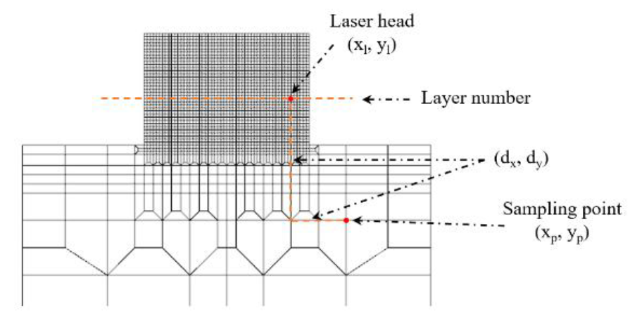
Fig. 2: The input features of the surrogate model

Overall, the input data consists in {𝐱_𝑗^(𝑖);𝑖=1,…,𝑁;𝑗=1,…,9}, where N is the number of configurations. Note that N = 19.9 million (2519 nodes × 1978 time-step × 4 simulation data) configurations as described above. The FFNN-based model is trained by optimizing the weights and biases W that exist inside the model. It is done by solving the mean squared error (MSE) problem for each iteration:

where, ℒ(𝑽), N_T and 𝑇^(𝑖) are the MSE loss function, training data and the temperature value corresponding to each configuration, respectively. Note that 𝑽 is the matrix of weights to be optimized, argmin is the argument of minimum and N_T=30%N is chosen for this task. The Adaptive Moment Estimation [10] algorithm is used in the stochastic gradient descent procedure to update network weights after each iteration based on training data with the learning rate of 0.001. In addition, to assess the performance of FFNN-based model, the metric of the coefficient of determination R² is used. It is defined as

where, M, T̂⁽ⁱ⁾,𝑇̅ and T⁽ⁱ⁾ are the number of samples, the predicted temperature from the FFNN-based model, mean temperature and actual temperature obtained by 2D FE model, respectively. Hence, the closer to 1 the value of R² is, the better the model predicts.

3 Results obtained from FFNN-based model

This section presents the prediction results obtained by the FFNN-based model. The analysis of the temperature results is based on three important points including the substrate (S) and the cladding (P) as shown in Fig. 3. Note that the cladding points P₁ and P₂ are located on the symmetric line of the component.

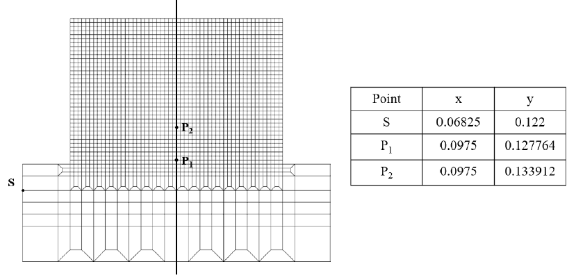Fig. 3: Position of three interest points at which temperature evolution is examined

Fig. 4 shows the train and validation losses of the model. It is observed that the training process ends at 300 epochs as the validation loss does not further decrease. Note that the epoch is the optimization step, Loss is the training loss per each epoch (see Fig. 4), Val_Loss is the validation loss per each epoch (see Fig. 4). The converged value of the validate set is chosen to correspond to a MSE lower than 5×10⁻⁵ as it is acceptable for the problem (see Fig. 4).

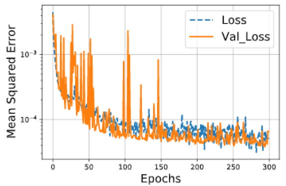Fig. 4: Training and validation loss of the FFNN-based model at each optimization step

3.1 Prediction of the temperature evolution of the DED process

Fig. 5 shows the temperature evolution for three interest points, namely S, P₁, and P₂ representative of the substrate and two different layers in the printed part. At each point, the temperature profile shows the characteristic cyclic thermal history related to the position of the laser head.

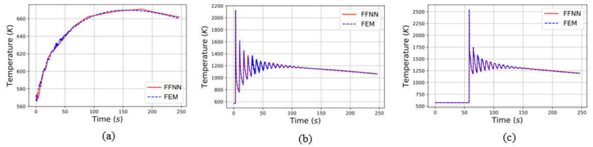Fig. 5: Temperature evolution predicted at 3 locations (a) substrate S, (b) Cladding P1 and (c) Cladding P2 by FE and FFNN-based models

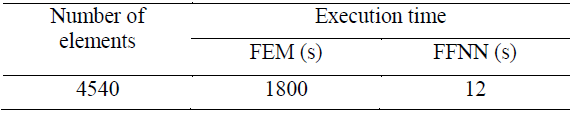
For the temperature evolution of the substrate S (see Fig. 5(a)), the result shows a good agreement between the temperature profile computed by the FFNN-based model and the FE model. It is noted that the 5 additional features named (v) to (ix) in Fig. 2 are set to zero for all the substrate points. This choice is explained by the observation that the substrate point S stays far from the laser head and its temperature value is not affected much by these additional features. Consequently, the prediction of the substrate point is just a function of the nodal coordinates and time. In detail, the substrate point has a R2 value of 0.995. Fig. 5(b) and Fig. 5(c) show the comparison of the temperature evolution of the cladding P₁ and P₂ obtained from FE and FFNN-based models. Similar to substrate S point, the temperature evolution of the two cladding points is predicted well by the FFNN-based model with a high R² value of 0.991 and 0.999, respectively. As shown in Fig. 5, the oscillations of the temperature profiles as well as the temperature peaks are well captured by the FFNN-based model. Table 1 shows the computational cost and output data size of the FE and FFNN-based models. As observed in Table 1, the time required to obtain the temperature history of the FEM simulation for 4540 finite elements is reported as 1800 seconds. On the other hand, the FFNN-based model only takes 12 seconds to get the results. In summary, the FFNN-based model outperformed the FE model in computing time once datasets and FFNN-based model are developed.

Table 1. Computational cost of FE and FFNN-based models

3.2 Prediction of the melting pool size

Fig. 6 shows the comparison of the melting pool size obtained from the FE and FFNN-based models. The melting pool size is the liquid zone generated by the laser. It is built by the powder flow melted by the laser energy as well as by the fusion of the previous build layers. The size of the melting pool plays an important role in determining the microstructure and mechanical properties of the printed sample. It is directly extracted from the temperature field data as the material points having a temperature higher than the melting temperature. As shown in Fig. 6, the predicted melting pool size is in good agreement with FE prediction with a R² value of 0.971. It is noted that the value of melt pool equal to zero means the laser is switched off. Similar to the temperature field prediction, the peak variations of the melting pool area with the height of the cladding are well captured by the FFNN-based model.

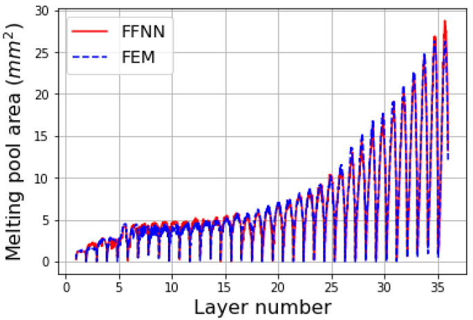Fig. 6: Melting pool area predicted from FE and FFNN-based models

3.3 Assessment of the FFNN-based model prediction

In this section, the assessment of the FFNN-based model prediction is performed to give an insight into the model performance. Given a very small amount of FEM simulation data, one needs to assess the predictive ability of the model compared with the case of a larger amount of FEM simulation data. Each FEM simulation data is created by changing the value of input energy 𝑄_𝑖𝑛𝑡∈[0.8,1.2] [Q₀]. At this stage, a total of 18 FEM simulation data is created instead of the 5 groups of Section 2, and then they will become the validation data of the FFNN-based model. The value of Q_int used to create FEM simulation data for training and validation of the FFNN-based model are described in Table 2. As shown in Fig. 7, the model predicts the other 18 FEM simulation data with a value of R² greater than 0.99 while the FFNN-based model is trained by only 5 FEM simulation data (see Table 2). Note that the datasets used in training are also used for validation. Accordingly, the FFNN-based model is able to predict the FEM simulation data created by the input energy 𝑄_𝑖𝑛𝑡∈[0.8,1.2] [Q₀] with excellent accuracy.

Table 2. The value of Q_int used to create FEM simulation data for training and validation of the FFNN-based model

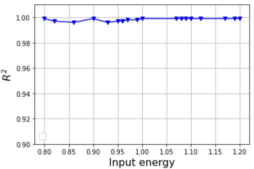Fig. 7: Assessment of the FFNN-based model prediction using R² metric

4 Conclusion

In this study, a simple FFNN-based surrogate model for the prediction of the temperature evolution and melting pool size in the DED process is developed. The numerical data of the evolution of the temperature fields under different process settings are obtained using a high-fidelity finite element model, which has been validated by experimental measurements. Beside the input energy, nodal coordinates and time, five additional features are considered as the input features of the FFNN-based model. Consequently, the surrogate model predicts the temperature evolution as well as the melting pool size of the DED process with excellent accuracies of 99% and 97%, respectively. In the future study, an optimization framework for the process parameters will be developed using Bayesian optimization.

Acknowledgements

This work was funded by Vingroup and supported by Vingroup Innovation Foundation (VINIF) under project code VINIF.2020.DA15..