1 Introduction

Additive manufacturing (AM) was devoted initially to prototyping. However, this process has become a serious competitor for the production of metal parts with technological evolution [1].

Wire arc additive manufacturing (WAAM) has become a promising alternative to conventional manufacturing processes due to its high deposition rate (1-4 kg/h) [2], environmentally friendly processes [3], productivity [4], cost reduction [1] and reduction in the buyto-fly ratio (from around 10-20 for a conventionally machined component to 1 for WAAM) [5].

There are a variety of WAAM technologies that can be classified in 4 groups depending on the welding generator used: gas tungsten arc welding (GTAW), gas metal arc welding (GMAW), cold metal transfer (CMT) and plasma arc welding (PAW) [6][7]. WAAM is a process that allows parts to be produced by successive addition of material in the form of layers composed of several weld-lines. The manufacturing of a part layer by layer presents a freedom of design. Therefore, this process allows the realization of parts with complex shapes [8] but heat transfer need to be evaluated before completion.

This process has distortion problems such as strain and crack formation [8][9][10] due to high gradient temperature field and high rate cooling. Numerical simulation of this process is hence necessary to evaluate temperature field. It can be link to strain and mechanical properties. The objective could be to optimize parameters on the deposition process using the numerical predictive tool. Modeling of WAAM process is a complex step. It is necessary to study the couplings between physical domains such as metallurgy, mechanics and thermic [11].

In this study, a model of the thermal behavior is developed. The process studied is the CMT (cold metal transfer) process. The main aim of this study is to determine the evolution of the temperature field during the deposition of three weld-lines (wall) and to analyze the thermal cycles of the weld-line.

2 Material and geometry specifications of the WAAM wall

The geometry of the base plate is shown in Fig.1 and the dimensions are 200x60x12 mm³.The wall is built in the middle of the base plate and in the direction of its length. The geometry of these weld-lines is modeled by a rectangular section. It is defined by the width and height of deposit to simplify the problem. The assumption is based on experimental results [12]. In this project, metallurgical transformations are not taken into account. To simplify the problem, the thermo-mechanical coupling can be reduced to a weak coupling, which takes into account only the influence of thermal loading on the mechanical behavior of the part to be manufactured. Hence the mechanical and thermal analysis can be dissociated[13][11]. The thermal analysis can be used as input data for the mechanical analysis (residual stresses and strains).

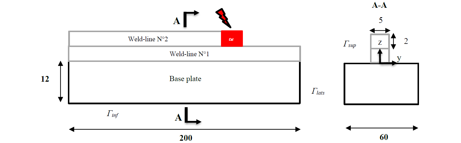
Fig.1. Geometry used to simulate WAAM process

In this study, three weld-lines are simulated. In the experimental work illustrated in literature studies[12], the first weld-lines have a width less than 5 mm. It is due to quick heat flow (base plate conduction and cooling system). The out heat flow becomes weaker and stable after few layers. However, according to J.Ding et al.[12], this change in width does not have a significant influence on the results. Therefore, a constant width and a constant height is used for all weld-lines.

The base plate is made of S355AR-JR steel. Its chemical composition is summarized in Table 1 and the chemical composition of the wire to be used is summarized in Table 2. This steel is widely used in AM. The high cooling rate does not influence strongly the mechanical properties [12].

Table 1. Chemical composition of the S355JR baseplate (in wt. %)

Table 2. Chemical composition of the consumable electrode (in wt. %)

2.1 Thermo-physical properties

In order to solve the equations for solid and liquid phase, it is necessary to define the thermo-physical properties (density, thermal conductivity, latent heat and specific heat). The same properties are used for the wall and base plate materials.

Thermal conductivity and specific heat depend on temperature. Work of Michaleris and Debiccari [14] is used as a reference to determine these thermo-physical properties. As shown in Fig.2, the specific heat decreases when the temperature is above 723°C due to phase transformation. A high thermal conductivity is used for temperatures above 1500°C.

A constant value of density is used in the numerical simulation (equal to 7860 Kg.m^-3). The latent heat of fusion is equal to 270 KJ.Kg^-1 between the solidus temperature (1450°C) and the liquidus temperature (1500°C) [14].

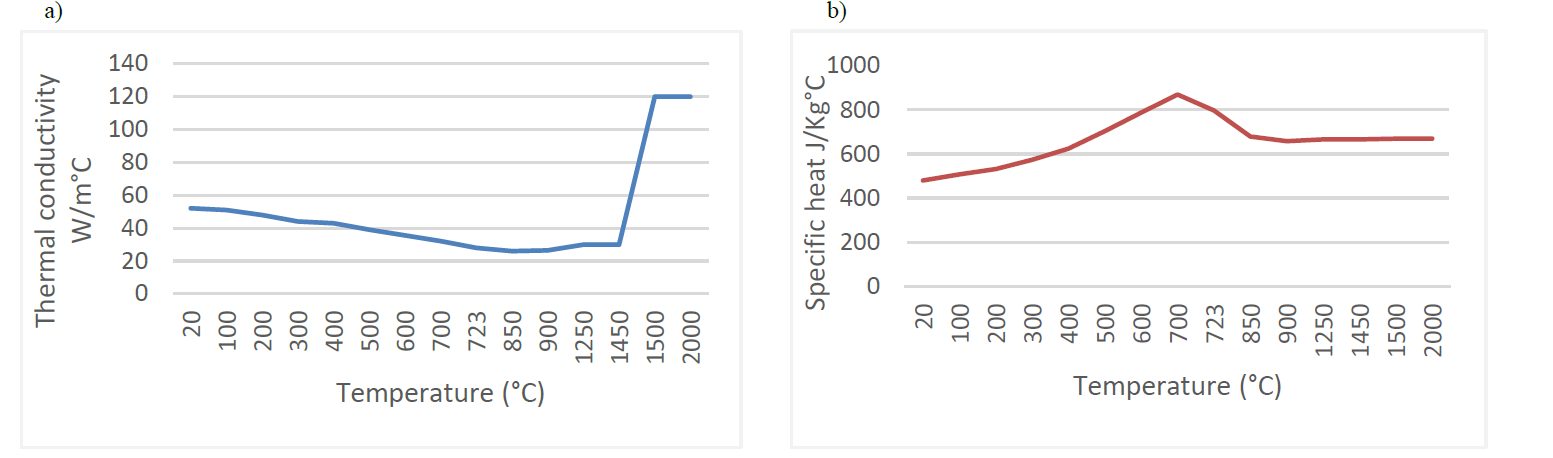
Fig. 2. Thermal properties of S355[14]: a) Thermal conductivity; b) Specific heat

2.2 Thermocouple positions

In the work of Ding et al.[12], temperature evolution is carried out from thermocouples placed during the experiment. The coordinates are shown Fig.3. Temperature variable were placed at the same position for the comparison between experimental and numerical studies.

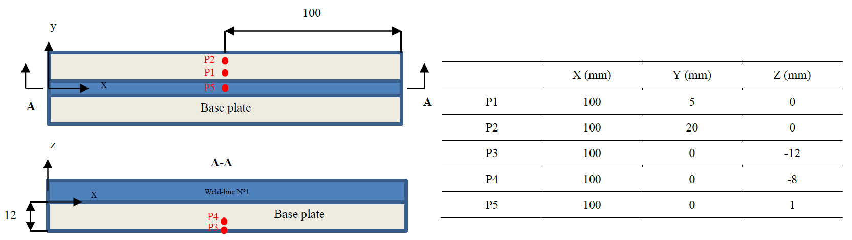
Fig. 3. The coordinates of the thermocouples[12]

3 Thermal finite element model

The numerical model is a transient FE analysis. The heat source is mobile in the x-axis direction and the workpiece remains fixed. It is based on the modelling of physical phenomena involved in the manufacturing process, such as heat transfer.

The finite element (FE) software ABAQUS is used to develop the thermal model. The objective was to have a predictive tool for temperature distribution which could be coupled to metallurgy phase or mechanical behavior (residual stress). Mesh is structured with linear hexagonal elements with 8 nodes DC3D8 (8-node linear heat transfer brick) [18]. A refined meshes are made in three areas since high thermal gradient:

• Along the x-direction, three elements were used to cover the length of the melt pool. The total number of elements along the direction of the deposit is equal to 80 elements with the size of 2.5 mm length.

• Along the y-direction, six elements were used to describe the melt pool with the size of 0.833 mm.

• Along the z-direction, three elements were used to describe the temperature variation with the size of 0.666 mm.

For the base plate, the constructed mesh is coarse since thermal gradients are low in this region. A representation is shown in Fig.4. The mesh dimension is optimized checking variance stabilization.

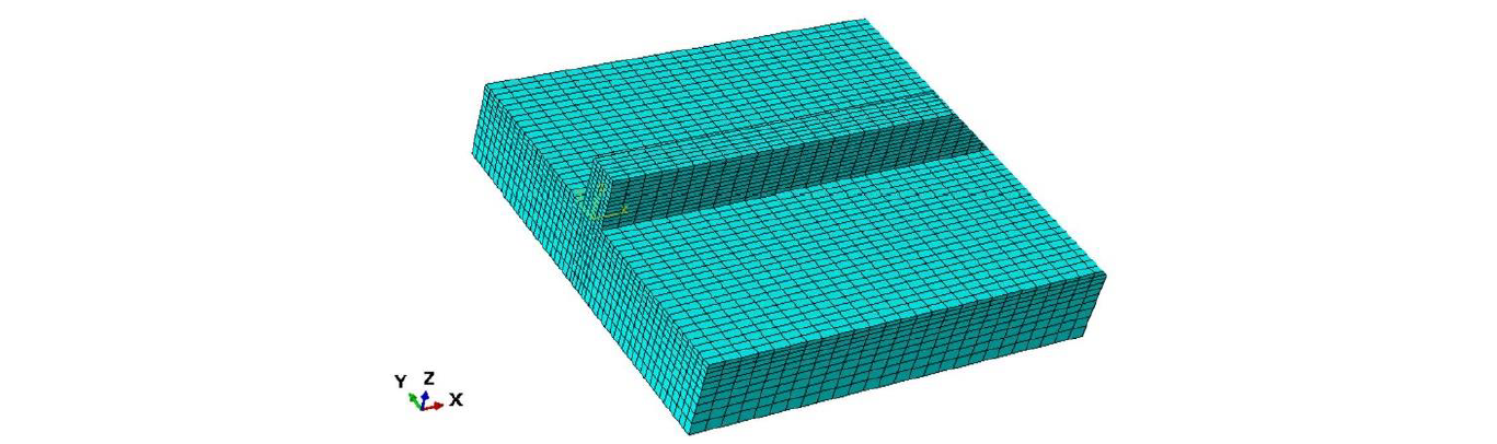
Fig. 4. The mesh of the transient model

The Finite-element activation strategy is used to simulate liquid material input. Initially, the wall is completely constructed of inactive elements, i.e. the mechanical and thermal properties are zero. An element is activated if it crosses the electric arc by attributing thermal and mechanical properties to it, otherwise it remains inactive [15]. This strategy has a disadvantage in terms of computational time but it allows a very realistic description of the process.

The liquid material deposition by electric arc is simulated as a volumetric heat source that moves along x-axis, based on Goldak's model (1), (2) [16]. This source is integrated with ABAQUS DFLUX subroutines.

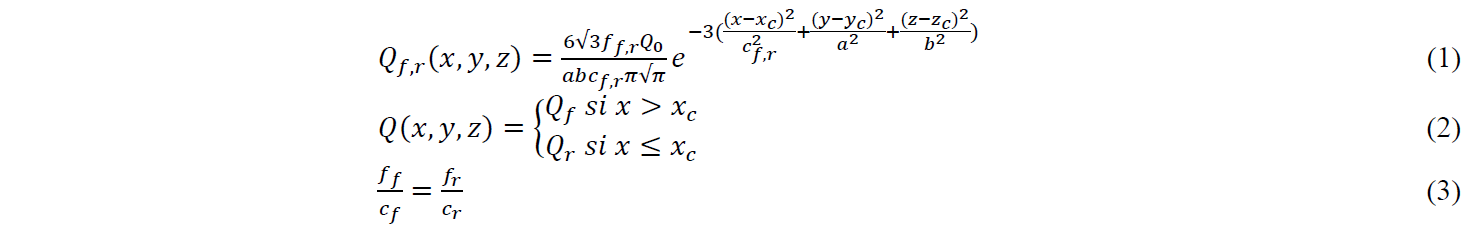
Where a is the width of the ellipsoid, b is the height of the ellipsoid, c_f is the length of the front ellipsoid and c_r is the length of the rear ellipsoid. f is a coefficient that allows to impose higher thermal gradients at the front of the torch than at the rear, f=f_f at the front

(x > x_c), f=f_r at the rear (x < x_c) with f_f+f_f =2. For reasons of continuity, a condition (3) should be imposed on the coefficient C which also takes 2 different values at the front and at the rear of the heat source [12].

The term Q₀=ŋ.I.U represents the maximum power where ŋ is the process efficiency, I is the current and U is the voltage, all parameters are summarized in Table 3.

Table. 3. Parameters used in the Goldak model[12]

During the deposition phase, the weld-line is introduced into the model using the element activation method with the 'MODEL CHANGE' option of ABAQUS. Initially, all steps are inactive (phase pre-step) and then the steps will be activated, step-by-step (weld line-i), by using an activation time, which depends on the welding speed. Smaller the size of the step is, closer the simulation results are to the experimental results but longer the computational time is. The size of the Step is equal to 10 mm and the activation time of each Step is equal to 1.2 second (For the inter-layer phase, the duration of the step is equal to 400 seconds, which is the inter-layer time required for a maximum temperature of 50°C. It is representative of a water-cooled aluminum machine plate. An organigram of the complete process is shown Fig.5.

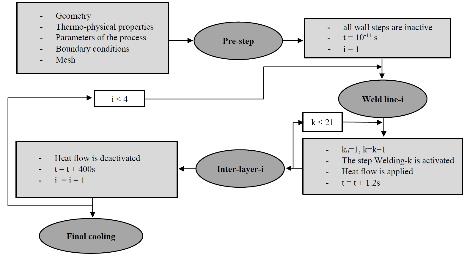
Fig. 5. Organigram of the numerical simulation

4 Results

A comparison between the predicted data obtained by this study and the experiment results of Ding et al.[12] is presented in Fig.6. It shows numerical transient and the experimental thermal histories at one of the measurement positions on the base plate (P1) that are shown in Fig.3. The predicted temperatures were extracted from the nodal points. The gap between transient model and experimental result is equal to 5.6 % for the first peak, 1.3 % for the second peak and 8.6 % for the third peak. Predicted heating and cooling rates are correlated with the experimental results. A comparison of the five positions will be discussed.

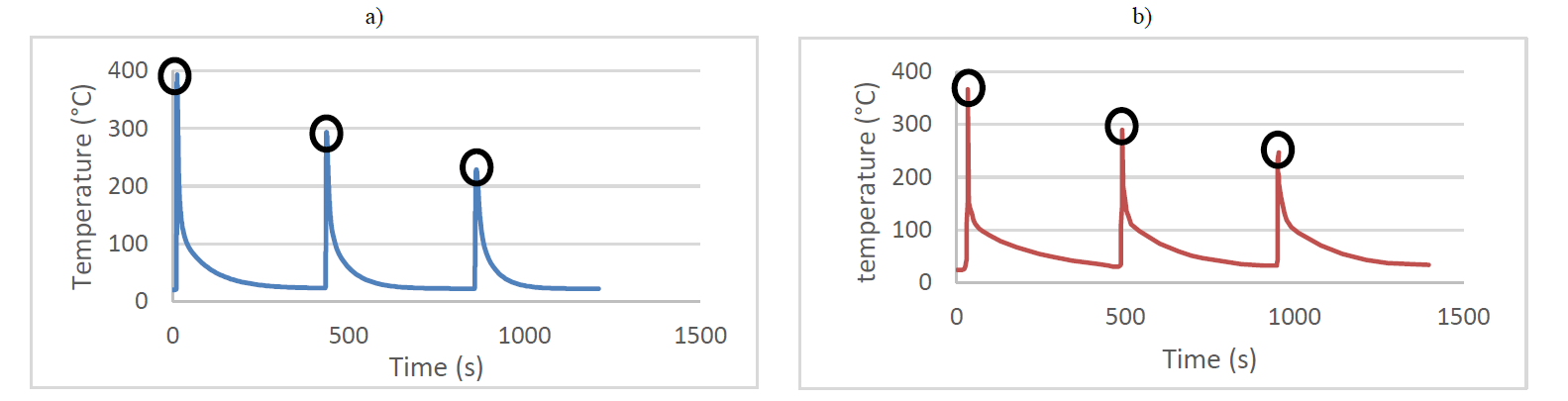
Fig. 6. Temperature verification on the measuring positions: a) Thermal cycle found by the transient model (P1); b) Thermal cycle detected by the thermocouple (P1)[12].

Transient thermal cycles at five points (Fig.7.a) located on a cross section (x=100; z=0) are illustrated in Fig.7.b. All point are equidistant, however the thermal gap decrease along the y-axis from ≈ 250°C between C₁ and C₂ to less than 30°C between C₄ and C₅. The thermal gradient decrease until it reaches a few degrees after 30 seconds.

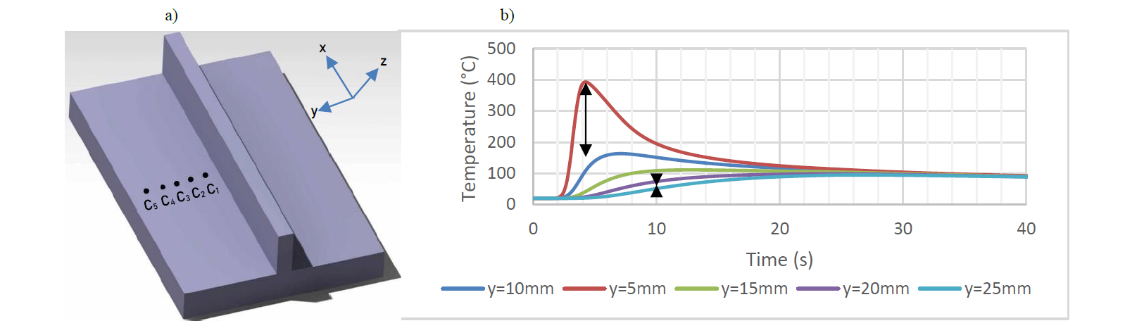
Fig. 7. Transient thermal cycles at different points located on a cross section perpendicular to the x-axis: a) Positions of measurement points; b) Transient thermal cycles.

The temperature cycles of eleven points (Fig.8.a) located along the weld-axis (y=0; z=0) are shown in Fig.8.b. The maximum temperature reached remains constant (≃2200°C) for all points after about 20 mm (distance travelled after the first 2.4 second of deposition) except the point at the end of the weld-line (x=200 mm), which corresponds to the extinction zone of the heat source. It reaches a slightly higher maximum temperature (≃200°C).

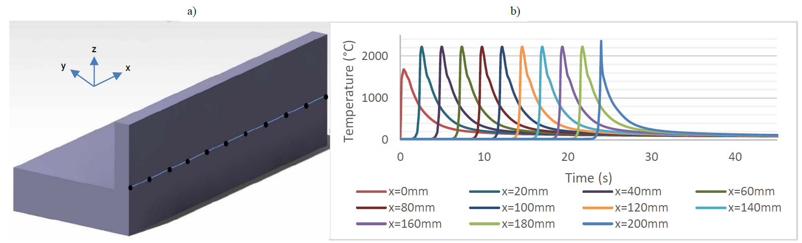
Fig. 8. Thermal cycles during the deposition along the x-axis: a) Positions of measurement points; b) Transient thermal cycles.

The thermal cycles at different heights of the deposited wall were acquired from the mid-length cross section (Fig.9.a) of the model, and shown in Fig.9.b. The maximum temperature increases after each deposition, it increases by 6 % between weld-line 1 and weld line 2, and by 3 % between weld-line 2 and weld-line 3. The peak of the first weld-line is lower due to the influence of the cooling system under the base plate.

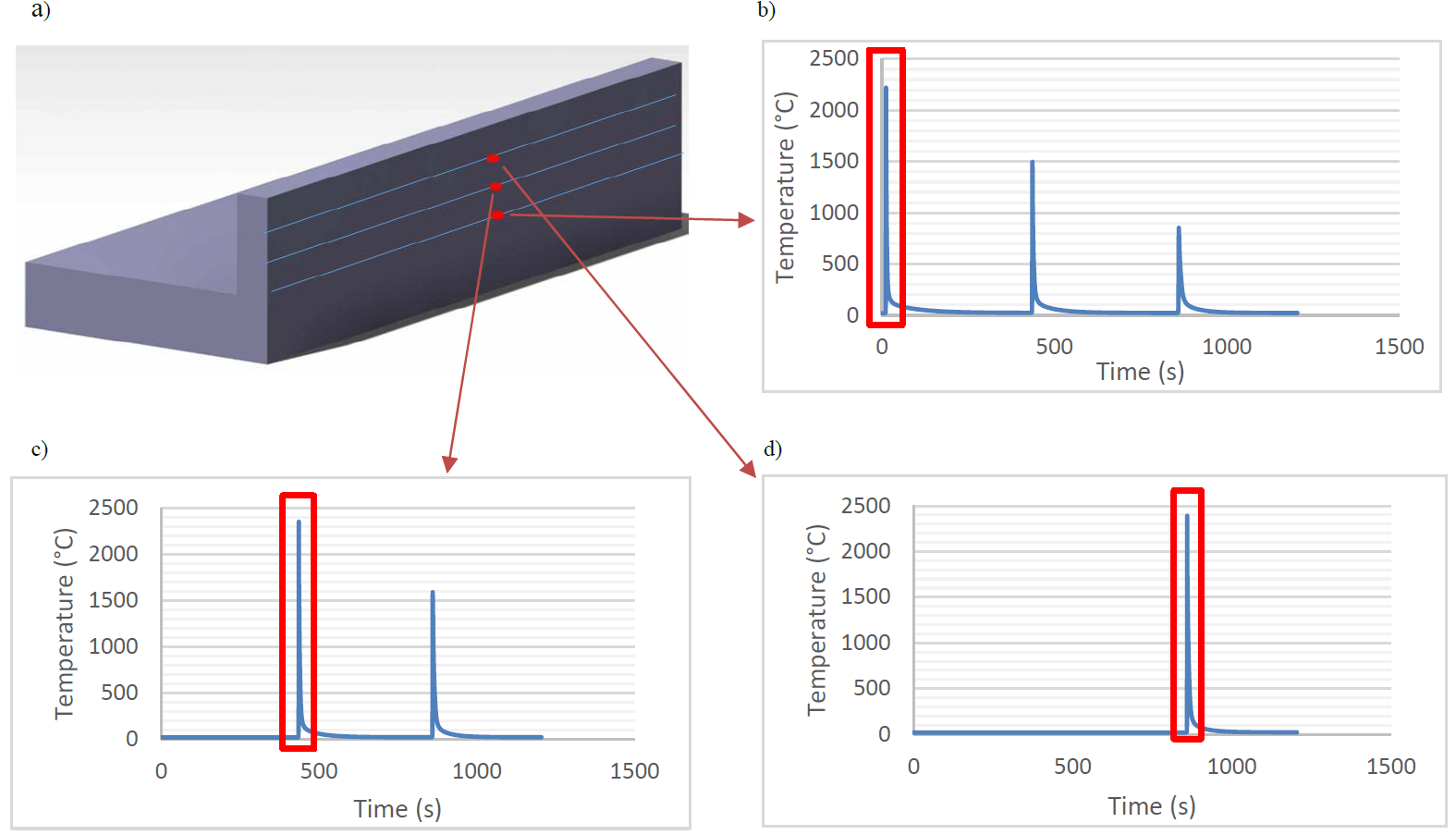
Fig. 9. Thermal cycles at different points located in the middle of the three weld-lines: a) Positions of measurement points; b) Thermal cycle in the middle of the first weld-line; c) Thermal cycle in the middle of the second weld-line; d) Thermal cycle in the middle of the third weld-line.

5 Discussion

The process starts at time t=0 s with an initial temperature equal to 20°C. Then the deposition phase begins, the heat source is applied, the temperature gradually increases at the front and the rear of the melt pool where the temperature is higher than the melting temperature of the material used (1500°C) as shown in Fig.10. A high thermal gradient is generated from the beginning of the deposition phase, in fact the maximum temperature varies from 20°C to 2300°C at the time t=0.298 second.

Fig. 10. Goldak double ellipsoidal heat source model

By analyzing the thermal cycles illustrated in Fig.6:

• A good concordance in the temperature rise during the deposition phase in the different measurement points.

• A similar evolution between the simulated temperatures and the measured temperatures.

• A slight difference between the maximum simulated and measured temperatures.

The comparison shows that the numerical model developed can predict the temperature evolution during the WAAM process with reasonable accuracy. Indeed, the Table 4 shows the temperature gaps |𝑇_{𝑡𝑟𝑎𝑛𝑠𝑖𝑒𝑛𝑡} − 𝑇_{𝑒𝑥𝑝𝑒𝑟𝑖𝑚𝑒𝑛𝑡𝑎𝑙}| between the transient model and the experimental results[12] in each point of measurement during the deposition of three layers. All gaps do not exceed 25°C except in the case of point P5, in which the gap reaches 150°C (21 %) during the deposition of the 3rd weld-line. This difference may be due to fluid mechanics phenomena which is not taken into account in this study[17].

Table 4. Thermal gaps

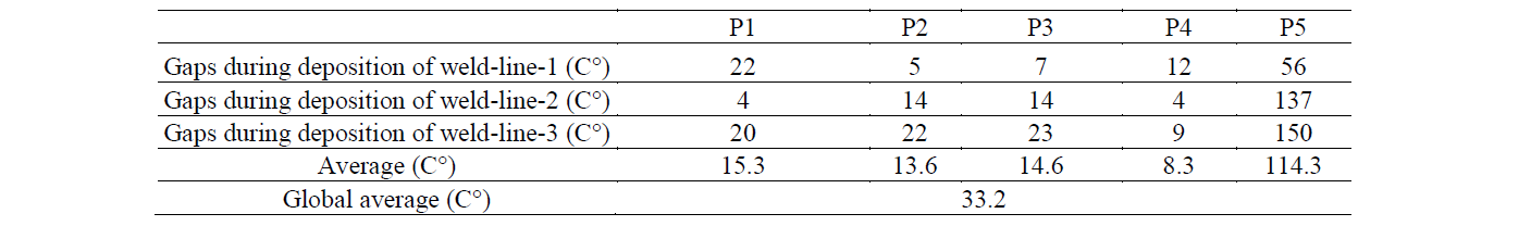
Fig.7 shows the temperature evolution as a function of time for five points located at different distances from the weld-line. It is noticeable that the thermal gradient is high in a cross section. This gradient decreases deeply after a few seconds, it is only a few degrees as shown in Fig.7. The farther the point is along the y-axis, the lower the maximum temperature reached. The maximum is reached after a higher time when the point is further away from the source. A similar thermal behavior has been shown by the experimental determination of the temperature evolution during welding presented by A.Ortega [5]. This delay is due to the variation of the heating speed along the y-axis.

Thermal cycles along the x-axis show that a quasi-stationary regime is established after a few seconds at a speed of 8.33 mm/s, where the maximum temperature remains constant, which explains the poor wettability at the beginning of the deposition [5] as shown in Fig.11. The maximum temperature reached for the point at the end of the first layer is higher than the maximum temperature reached in the quasi-stationary regime due to edge effect.

Fig. 11. An example of a WAAM sample fabricated using mild steel wire

Fig.9 illustrates the thermal cycles recorded in the middle of the three deposited weld-lines. It is noticeable that the maximum temperature increases progressively until it reaches about 2480°C during the 3^rd weld-lines. According to previous research [2] the maximum temperature stabilizes after 10 - 15 layers. Indeed, heat transfers by convection and radiation balance the heat input generated by the electric arc.

6 Conclusion

A thermal model was developed and compared with experimental results. The objective was to validate the model as a predictive tool. The results present the temperature evolution during the deposition phase, the inter-layer phase and the cooling phase. The evolution of the thermal gradient layer by layer can be analyzed. The simulation showed that:

1. Transient models can accurately predict the heating and cooling cycles compared to experimental results.

2. A quasi-stationary regime is established during each layer after a few seconds (3-5s), during which the temperature field is stable. Deposited layer keeps hence the same height and width.

3. The instability of the melt pool at the beginning of each layer leads to an accumulation of material or a ‘macro-drop’ which causes a poor wettability.

4. The superposition of layers generates a temperature increased layer by layer.

5. At a cross section, the high thermal gradient decreases quickly after few seconds.

Finally, this thermal model can be carried out for thermo-mechanical prediction, in order to analyze the evolution of the residual stresses and strain.