1 Introduction
The current industrial context encourages the optimization of resources in production processes [1]. Particularly in the processes of forming and machining metal parts, the reduction of energy and raw material are key points to increase such efficiency.
During the last decades, numerical simulations have become an indispensable tool in the study of mechanical manufacturing processes. Through accurate simulations, empirical-based operations, costs associated with trial and error, and wastes of raw materials can be reduced.
However, the study of the interactions of different processes in a production line continues to be a challenge, as they have not been well characterized in a global manufacturing process chain. The processes are generally modeled separately without integrating their interactions and the material history. The release of internal stresses generated on earlier stages of the manufacturing process can lead to undesirable deformations in the part being manufactured. This usually leads to intermediate processes of residual stress removal by means of an annealing process, which requires a considerable amount of energy.
The vast majority of numerical simulations are based on an isotropic hardening evolution of metal (i.e[2]–[4]). Kinematic, combined or anisotropic hardening models are restricted almost exclusively to the study of cyclic phenomena, such as fatigue (i.e [5]–[8]). This work proposes to study the influence of the hardening rule in order to follow the history of the evolution of the thermodynamic state variables that characterizes the metal during the global manufacturing process.
Qualitative and numerical examples are carried out by using different hardening rules, in order to evaluate differences in the prediction of the metal response for the same loading history. This difference has implications from both the energy point of view and the final equilibrium point of the manufactured metal part (state variables). The analysis suggest that the anisotropy induced during strain hardening has effects that should not be neglected in a global simulation of a mechanic part manufacturing process.
2 Domain of validity
This work seeks to establish the influence of the choice of hardening rule along a loading history. Viscous and thermal effects are not covered. Considering this hypothesis, the validity of domain is limited to the study of the following [9]:
-
Low temperature usage, up to a maximum of one quarter of the absolute melting temperature.
-
Damage absence. Loads and strains must remain below around half of the fracture load. For cyclic loads, it is applicable if the number of cycles remains below the corresponding stabilization value.
3 Thermodynamic theoretical frame
During strain hardening phenomena, each material particle has its own loading history and will develop new hardening characteristics a as function of it. The use of isotropic behavior rule (the most commonly hardening rule used on manufacturing procedures simulations), may lead to an underestimation of plasticity phenomena during a multiple step manufacturing process with different orientation of solicitation, as it will be demonstrated later.
It is possible to characterize the transformation process undergone by the material by considering each element as a thermodynamic system.
When plasticity occurs, part of the absorbed energy is dissipated to the environment as a heat and the rest is devoted to generate a change in the structure of the metal (change of phase, dislocations, etc) [9], [10]. This phenomenon can be described as the evolution of a thermodynamic process.
A thermodynamic state is a condition that is fully identified by a set of parameters known as state variables. The challenge then of characterizing the strain hardening phenomena as an evolution of the thermodynamic state, is to identify the state variables and to model their behavior. On the other hand, this approach ensures that a unique set of variable characterize a specific thermodynamic state, independently of the load history.
From the first and second principle of thermodynamics the Clausius-Duhem inequality is written as[9]–[11]:

where 𝜎 represents the stress field tensor, 𝜀̃ the strain tensor, 𝜓 the specific Helmholtz free energy, 𝑠 the generated entropy, 𝑞 the heat flux tensor, T the temperature. For reasons of the scope of this work described in section §2, only the first two terms are considered.
The free energy is a function of the state variables 𝛼i associated to hardening phenomena used to describe the plasticity. Any variation is expressed as:

Due to the scope of this work only the second term on the right side of the equation is considered. The variation of the free energy due to a change of a state variable is known as the specific hardening force:

The nature of the different hardening forces ( 𝐴 ) adopted in the model defines the hardening rule used in the behavior law. For example, an isotropic model uses a scalar variable ( 𝑅) that represents an expansion of the elastic boundary. In a kinematic model the thermodynamic force is given for the displacement of the elastic boundary, called backstress and is represented by the tensor 𝑋. As result in this modelling, the loading direction has a significant effect on multiple load steps and in non-proportional loading.
As the matter of fact, observed phenomena cannot be described accurately only with a single hardening force. Combined models use both variables (the isotropic and the kinematic) to describe the evolution of the elastic threshold during a plastic flow, some of these models are described in [6], [7], [12]. Furthermore, several works details an anisotropic evolution of the elastic limit where a distortion of the elastic threshold is verified [8], [13]–[24]. However some observations differ from one author to another and most of the studies are not integrated in the thermodynamic framework developed by Germain[11]. More studies should be carried out to clarify the anisotropic evolution of the elastic threshold.
The free energy modelling does not limit the number of thermodynamic forces used to describe the evolution of the state, more variables may be added to describe the distortion of the elastic threshold.
4 Plastic flow
There are two conditions that should be satisfied to consider that a specific load has reached the plastic regime. The first one is that the load function must be equal to zero [9], [10]:

The load function 𝑓 depends on the stress tensor, the hardening variables 𝐴 (also called thermodynamic forces before) and material constants. This function relates a set of tensorial variables to a scalar value; this value is negative when the load corresponds to the elastic regime ( 𝑓 ≤ 0). So, the fact that 𝑓 = 0, does not guarantee the plastic regime yet, since it only means that the load is found in the elastic/plastic frontier.
Therefore, equation (4) represents the elastic frontier or elastic threshold. The load function cannot take values greater than 0, so when an external solicitation is found outside of the elastic domain it will induce a modification of the elastic threshold by following the consistency condition :

and the elastic threshold will continuously evolve until the first condition (equation 4) is finally satisfied.
5 Flow rule
In order to ensure the uniqueness of the response of a defined thermodynamic state [11] due to an external solicitation, it is necessary to establish the flow rule that states the rate of change of the thermodynamic variables( 𝜀̃ , 𝛼 ):
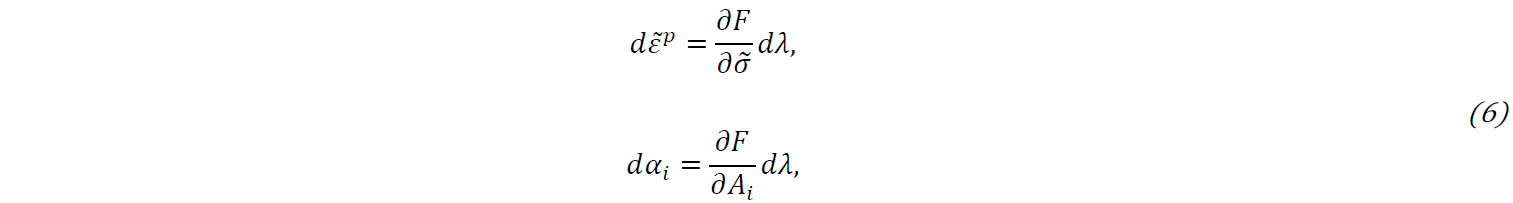
where the function 𝐹 is a function of the stress components and the strain hardening variables 𝐴i and 𝜆 is a scalar known as the plastic multiplier.
To fully describe a behavior law on a thermodynamic framework, it is necessary to model the free energy 𝜓 as function of the thermodynamic variables, the load function 𝑓 and the flow potential 𝐹.
Thus defined, 𝐹( 𝜎, 𝐴i ) is a flow potential that controls the evolution of the thermodynamic state variables through the equation (6), while f is the potential that defines the elastic boundary [9], [10].
6 Hardening rule families
The hardening rules that describe the behavior laws may be classified by the hardening rule criteria in four mean families; isotropic, kinematic, combined and anisotropic. Each family is characterized with a specific hardening variable or set of variables (with the exception of the anisotropic family that may include non-conventional hardening variables).
Isotropic hardening laws are characterized by a scalar hardening variable (usually represented by 𝑅). In this particular family, hardening evolves evenly in all directions when the elastic threshold is reached, are interpreted as an expansion of the elastic domain [9], [10]. Therefore it is not possible to model some phenomena that could have a relevant importance in the simulation of the manufacturing process chain interaction, such as the generalized Bauschinger effect.
Kinematic hardening rules, model the strain hardening phenomena as a translation of the elastic threshold instead of an expansion, the coordinates of the center of the elastic domain represents the hardening variable (a tensor usually represented by 𝑋) [5], [6], [9], [10], [25]. This kind of modelling allows to reproduce the Bauschinger effect and the ratcheting effect on cyclic loads, a review and evaluation of different kinematic hardening rules are given on [6], [7]. The translation of the elastic threshold induces an anisotropy on the state of the metal.
The combined hardening rule refers to the use of kinematic and isotropic hardening variables. The use of both variables allows to reproduce cyclic hardening and softening which would not be possible by using only one hardening rule [6], [9], [10].
Experimental studies show that a more complex hardening rule is needed to accurately reproduce the strain hardening effects such as the Bauschinger effect, cyclic hardening and softening, ratcheting effect, etc. [6], [9], [10], [21], [26]. An anisotropic deformation of the elastic threshold is found during a plastic deformation, the loading direction plays a major role in the adopted shape. Only a few of these models [23], [26] are included in thermodynamic framework presented, further studies are needed in order to evaluate if their application show relevant differences in relation to kinematic or combined models.
7 Practical example
As previously stated, during the manufacturing process, each particle of a part is subjected to combined loads. In the context of the study, for example the manufacturing process involves successively a rolling and a machining process by removing material. For these two processes, the rolling method will generate a high compressive stress with residual deformations and during machining the material will undergo both shearing and localized compression. Between two consecutive steps, there is a loading release process. The stresses developed in the load release are generally within the elastic behavior regime.
The kinematic and combined hardening rules are models consecrated mostly to the study of cyclic loading, in order to describe the Bauschinger effect, cyclic hardening and softening, etc.
The present example aims to highlight the implications of modeling the Bauschinger effect (by a kinematic hardening rule) during a sequence of consecutive loads under different directions, normally neglected (isotropic model).
To simplify the study and to represent a loading history under plastic deformation, three loads are chosen that exceed the initial elastic limit, under combined stresses of different directions, respecting the domain of validity of the work in a theoretical framework.
These loading paths do not represent the stresses during a specific process, but the results will serve to draw conclusions regarding the importance of the role of the hardening rule during the simulation of a global process.
7.1 Problem statement
In order to show the influence of the hardening rule on the results obtained after a chain of multiple loading steps, the isotropic and kinematic laws presented on table 1 are considered, where 𝑆 is the stress field represented on the deviatoric space:

Elastic strains are calculated using Hooke’s law with an elasticity modulus of 𝐸 = 200 ( 𝐺𝑃𝑎) and Poisson’s coefficient equal to 𝜈 = 0.3.
Table 1. Behavior laws constitutive equations. Extracted from [9]
![Table 1. Behavior laws constitutive equations. Extracted from [9]](docannexe/image/4049/img-8.png)
A particle is submitted to three different consecutive loading steps, arbitrarily chosen under the condition of forcing a plastic hardening in the kinematic model, respecting the domain of validity of this work. The loading history is summarized on table 2:
Table 2. Loading steps description (Units given in Mpa)

where 𝜎eq refers to the Von Mises equivalent stress.
7.2 Results and analyses
Table 3 shows the strains obtained after each loading step as well cumulated plastic strain ( 𝑝cum ), calculated with both considered behavior rules.
During step A no major difference is noted on the response stress vs. strain, however the modelling on strain hardening brings an important consequence for later stages. Figure 1a) helps the comprehension through a schema. Both models predict yielding at the same moment when the load reaches the elastic threshold at point a. The final solution (strains) is similar in this case only because yielding occurs at same moment and at the same point.
The last case is going to be true only for an annealed state, free of hardening effects. The residual properties of the metal affect the subsequent loads.
The load B has the same equivalent stress value of load A (150 Mpa), consequently there is no yielding when the isotropic model is used. This is clearly reflected on plastic strain values at the end of step B, where there is no change compared from those obtained on step A. On the other hand, the kinematic model yields when the loading path reaches the elastic threshold at the point q on figure 1b.
Table 3. Strains comparison along a multistep loading process of isotropic and kinematic hardening rules response
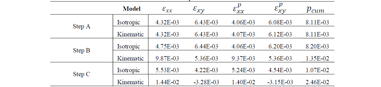
On step C (represented schematically in figure 1c) the load path BC intercepts the kinematic threshold model on 𝑞′ and the isotropic on 𝑡. Again, a longer portion of the load is on plasticity on the kinematic model compared to the isotropic. As one of the consequences, the final strain on the kinematic model exceeds the isotropic on 162% on the principal direction and they differ of the sign on the shearing direction.
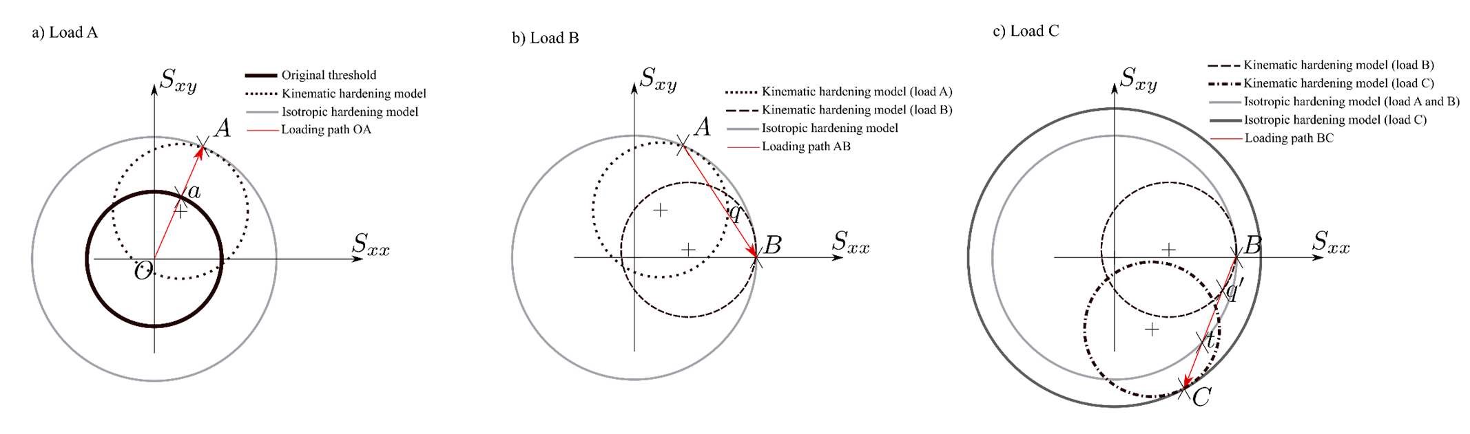
Fig 1. Schematic representation of strain hardening effects on the elastic threshold during the loading process. a) Loading step A. (b) Loading step B. (c) Loading step C
The predicted plastic energy developed during strain hardening shows also an important discrepancy between the two models as shown in table 4. The specific plastic energy developed during strain hardening may be calculated by:

The kinematic hardening model predicts after the three loading steps a total specific energy of (3.22 𝑀𝑝𝑎. 𝑚𝑚/ 𝑚𝑚) while the isotropic model only predicts 1.43 ( 𝑀𝑝𝑎. 𝑚𝑚 / 𝑚𝑚). Again, the difference between predictions is over 100%.
The dissipated energy is the difference between the specific plastic energy developed during strain hardening and the free energy 𝜓[9]. So the dissipation will also differ on the overall process.
Table 4. Specific energy developed

The results show that strain hardening and thermodynamic variables have a major importance on describing the state of the material.
Isotropic models are not capable to reproduce the generalized Bauschinger effect, so is expected its incapability to reproduce properly a chain of consecutive loadings. This also may be explained by the fact that isotropic model are based on monotonic tests, following a single load.
The kinematic model used in this work corresponds to the Amstrong and Frederick model [5], according to Portier et al [7] it over estimates the Bauschinger effect. Further studies should be carried out to compare results obtained with different kinematic, combined and anisotropic models. The residual stress field found on a work piece may be compared to the results of simulations performed with the different hardening rules as a methodology to evaluate the accuracy of each model
8 Conclusion
A considerable amount of energy may be reduced on manufacturing process if simulations are accurate on predicting the effects of one manufacturing process on subsequent stages, optimization algorithms may be implemented. In order to look for a methodology capable of ensuring a traceability of the state of the matter along the whole manufacturing process, the evaluation of a hardening rule presented on thermodynamic framework is revised.
The use of a behavior law in the thermodynamic frame allows establishing the relation between its thermodynamic state with its hardening state, assuring the unicity of the solution. So a defined state may be characterized by the stress, strains and the hardening variables.
Isotropic behavior laws are obtained through monotonic tests with annealed test tubes; they are accurate defining the stress/strain evolution along one single loading path. The generalized Bauschinger effect cannot be reproduced with this family of hardening rule, so it may be concluded that the thermodynamic state is not accurately defined. This situation leads to erroneous results when subsequent charges go through the elastic threshold (re-entering into elastic domain) on a multiple-step loading, which represents the most general case on a multi-step manufacturing process.
The practical example developed in this work offers an idea about how different results can be when using different hardening rules.
In general isotropic models will underestimate plastic strain hardening and dissipated energy on a multiple loading and nonproportional loading case.
Results must be compared with other hardening rules (kinematic, combined and anisotropic) in order to evaluate the accuracy versus cost of computation.
Future works foreseen to carry out simulations of a global process taking into account the conclusions of this work.
The present study does not take into account viscous, temperature and damage effects. Further studies should be carried out to include these effects in the model as well the state variables identification and modelling in order to create a complete phenomenological behavior law.
