1 Introduction

Fiber reinforced thermoplastic composites have garnered interest as they can have mechanical properties comparable with thermoset composite while allowing additional possibilities in part fabrication such as welding or reshaping. They also have the advantage of permitting reuse and recycling to a certain extent. However, since the thermoplastic matrices have both a high melting point and a high melt viscosity, their use has been mostly limited to long and expensive process such as autoclave or hot press. In order to be able to use faster and less energy consuming processes like the resin transfer molding process (RTM), reactive systems for thermoplastic synthesis have been considered. For instance, as the reactive mix for polyamide 6 (PA6) is based on the ε-caprolactam monomer, it has very high fluidity adapted to liquid composite molding processes (LCM) with fast in-situ polymerization of the thermoplastic matrix [1].

Hence, the intricacies of the synthesis has been the object of a number of past studies [2,3] because of the viscosity dependence to polymerization and crystallization, and the exothermic nature of the reaction. There are all phenomena susceptible to affect the impregnation of the fiber preform and the overall quality of the composite especially when considering dual-scale flows. Indeed, the inter-tow flow reaches each tows at different stages of the synthesis. As shown by Imbert et al. [4], the intra-tow flow itself is also transient but on a different time scale with storage and release of resin. In a recent study, Vicard et al. [5] used differential scanning calorimetry (DSC) to gather experimental data on a reactive mix with suitable synthesis duration for LCM processes. This has highlighted the different synthesis characteristics with relation to temperature and allowed the identification of a modified Hillier coupling of polymerization and crystallization model.

In this study, the rheology of the reactive mix is investigated using a plate-plate rheometer in order to evaluate the behavior of the viscosity during the synthesis, and precisely measure its initial viscosity at high temperatures. Then, a preliminary modelling procedure to simulate the flow of the reactive mix is presented. It integrates the polymerization kinetics from Vicard et al. [5] and the rheokinetics proposed by Davé et al. [6]. A simulation illustrating the modelling procedure is showcased.

2 Experimental study of the rheology

2.1 Reactive mix

The reactants used for PA6 polymerization in the rheological study comes from components provided by Brüggemann Chemical, Germany which are detailed in Table 1. The ratio of both the catalyst and the activator is defined at 0.79/1.10mol.% of the monomer, which was previously studied in order to determine its polymerization and crystallization kinetics [5]. To ensure minimal inhibition from humidity, the reactants are dried before use. The mix has been prepared by melting, stirring, and quenching using liquid nitrogen. The reactants in a dry atmosphere confined in a glovebox and the samples were subsequently stored in sealed containers.

Table 1. Components of the PA6 reactive mix

2.2 Rheological measurement setup

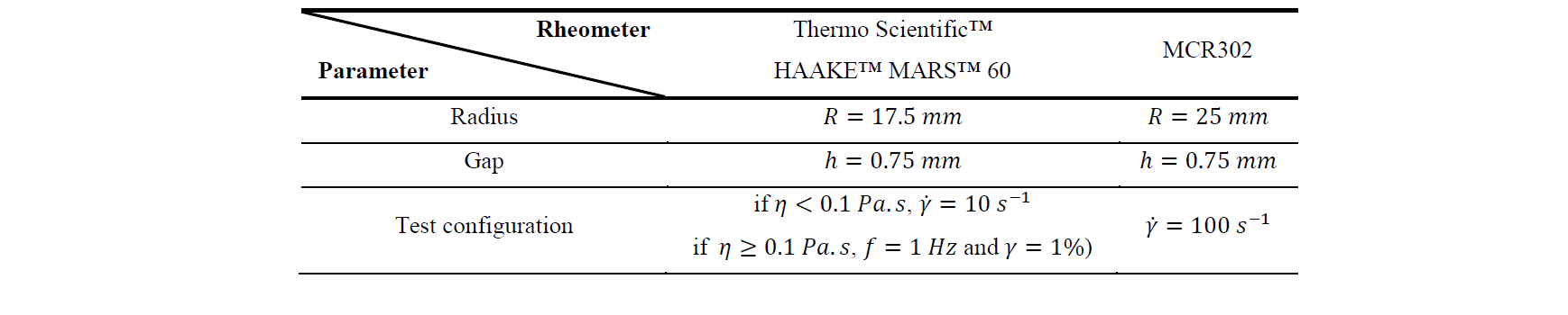
The rheological measurements were carried out thanks to a Thermo Scientific™ HAAKE™ MARS™ 60 plate-plate rheometer and a MCR302 plate-plate. Their configurations are described in Table 2, with 𝑓 the frequency, 𝛾 the deformation, 𝜂 the dynamic viscosity, and 𝛾̇ the shear rate. In order to limit the influence of shear stress on polymerization, the HAAKE™ MARS™ rheometer was configured to start with rotational shear before switching to oscillatory shear when the viscosity reaches 0.1 Pa.s. The MCR302 plate-plate rheometer was configured with high rotational shear in order to obtain precise measurement at very low viscosities approaching water viscosity.

All the experiments started at a temperature between 353 K and 383 K, at which the reactive mix is in liquid state without polymerizing. The sample is then heated at around 20 K/min until it reaches 453 K and is then maintained at this temperature until the end of the test. In order to avoid inhibition of the reaction by humidity in the air, the measurement unit is enclosed in a box fed with nitrogen.

Table 2. Configuration of the rheometers

2.3 Isothermal rheology at 453 K

Fig.1 shows that at 453 K the resin viscosity is directed by two growth regimes which are caused by the different time spans of the polymerization and the crystallization during the PA6 synthesis. Indeed, at 453 K the polymerization and the crystallization occur successively, which makes the lower slope between the two growth regimes the mark of the transition between these two phenomena [5].

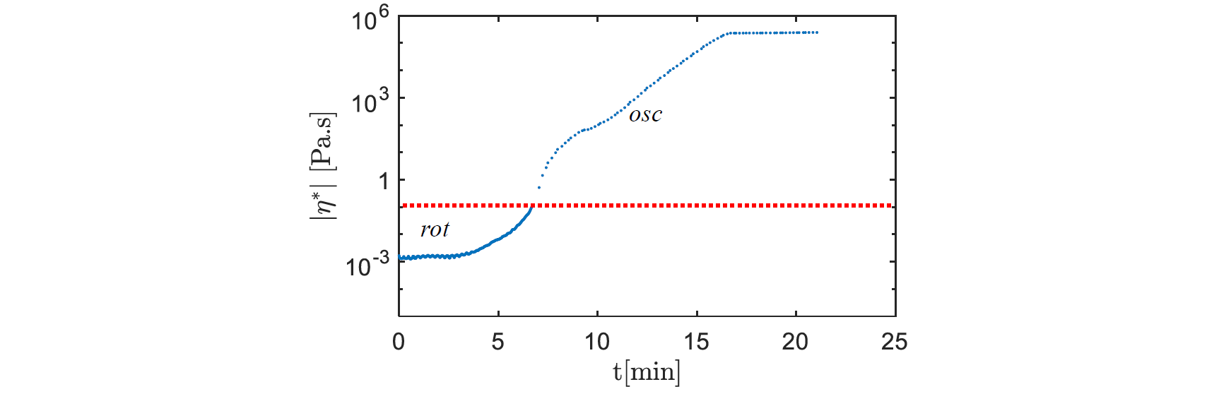
Fig. 1. Isothermal viscosity rise during conversion at 453 K

However, the viscosity rise occurs in a longer time span (around 16 minutes), than the expected duration of the synthesis (around 10 minutes [5]). This could be caused by the initiation time observed at the start of the measurement between 0 and 4 minutes which need further investigations. It is most likely explained either by the shear stress applied at the start of the experiment and/or lingering humidity, which may be inhibiting the reaction speed.

2.4 Temperature dependence of the reactive mix

As Fig. 1 shows, there is an induction time before the polymerization starts and raises the viscosity. Hence, the viscosity measured at high shear rate (𝛾̇ = 100 𝑠⁻¹) during the reactive mix heating can be used to fit a model based on well-known Arrhenius law (1) as shown in Fig. 2. This model can be used in order to simulate the temperature dependency of the initial viscosity before PA6 synthesis. The parameters are determined using the nonlinear least-squares solver integrated in Matlab^® Optimization Toolbox^TM. The results obtained are coherent with the laws that can be extrapolated from viscosity data of the molten monomer at temperatures lower than 403 K [6,7,8].

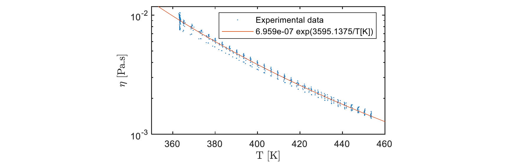
Fig. 2. Experimental viscosity measured during the reactive mix heating compared to the fitted Arrhenius law

3 Numerical simulation

Numerical simulations of the PA6 flow have been performed using OpenFOAM®, an open-source computational fluid dynamics toolbox using a framework similar to the one used by Nagy et al [9].

3.1 PA6 flow modelling

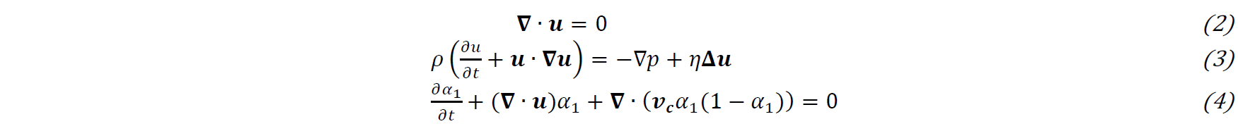
A biphasic model is used to model the flow of the reactive mix in the air. It uses the continuity equation (2) and the momentum equation (3) of the Navier-Stokes equations. The front is tracked using the volume of fluid (VOF) method (4) with an interface compression term where 𝒗𝒄 is the relative velocity between the two phases [10]. In these equations, 𝒖 is the velocity field shared by both phases, 𝒑 is the pressure, 𝜂=𝛼₁𝜂₁+𝛼₂𝜂₂ is the dynamic viscosity and 𝜌=𝛼₁𝜌₁+𝛼₂𝜌₂ is the density of the phase in an element.

The conversion to PA6 is followed by the transport equation (5) of the polymerization 𝑎, in which the rate of polymerization 𝑎̇ uses the Camargo version of Malkin’s Model (6), where 𝐴₀ is a constant representative of molecular collisions, 𝐵₀ an autocatalytic parameter, 𝑛_𝑝 the reaction order, 𝐸_𝑎 the activation energy and 𝑅 the universal gas constant.

The viscosity is modelled using a phenomenological law (7), where 𝐾_𝜂 was experimentally determined by Davé et al. [6] and deemed accurate when 𝑎<0.5. 𝜂₀ calculated at an isotherm using equation (1).

3.2 Computational method

The numerical method used to solve the aforementioned equations is adapted from the PISO (Pressure Implicit with Split Operator) algorithm in OpenFOAM®. It is a segregated second order accurate pressure-based solver that calculates the pressure and the velocity for transient flows [11]. The viscosity calculation and the polymerization equation are between the calculation of the VOF transport equation and the Navier-Stokes equation. The equations are discretized using the Finite Volume Method, with second order precise discretization schemes: the Crank₋Nicolson scheme is used for time discretization and the Van Leer scheme [12] is used for both the VOF and the polymerization transport equation advection term. In the Navier-Stokes equations, the diffusion term uses central differencing while the convection term uses the “limitedLinearV” scheme native to OpenFOAM® adapted for vector fields and blends central differencing and upwinding method in a way that satisfies TVD (Total Variation Diminishing) conditions for stability and convergence [13]. The time step Δ𝑡 is chosen adaptively, according to the maximum local Courant number (8) in an element with Δ𝑙 being its characteristic length. The maximum Courant number is chosen at 0.1 in order to ensure accuracy.

3.3 Preliminary simulation of the reactive mix injection

The flow domain is composed by a right-angled parallelepiped which constitute the injection domain and a cubic inlet located under the parallelepiped. Their dimensions and meshing are detailed in Table 3 and the geometry is shown Fig.3.

At the inlet, the conversion 𝑎 and its rate 𝑎̇ is defined at 0 while the phase of the reactive mix 𝛼_{𝑟𝑒𝑠𝑖𝑛} is defined at 1, inflowing with a speed of 0.003 𝑚∙𝑠⁻¹. At the outlet, a gradient of zero is defined for all fields. The pressure is defined as constant in the whole domain.

Table 3. Dimensions and meshing of the simulation domain

-

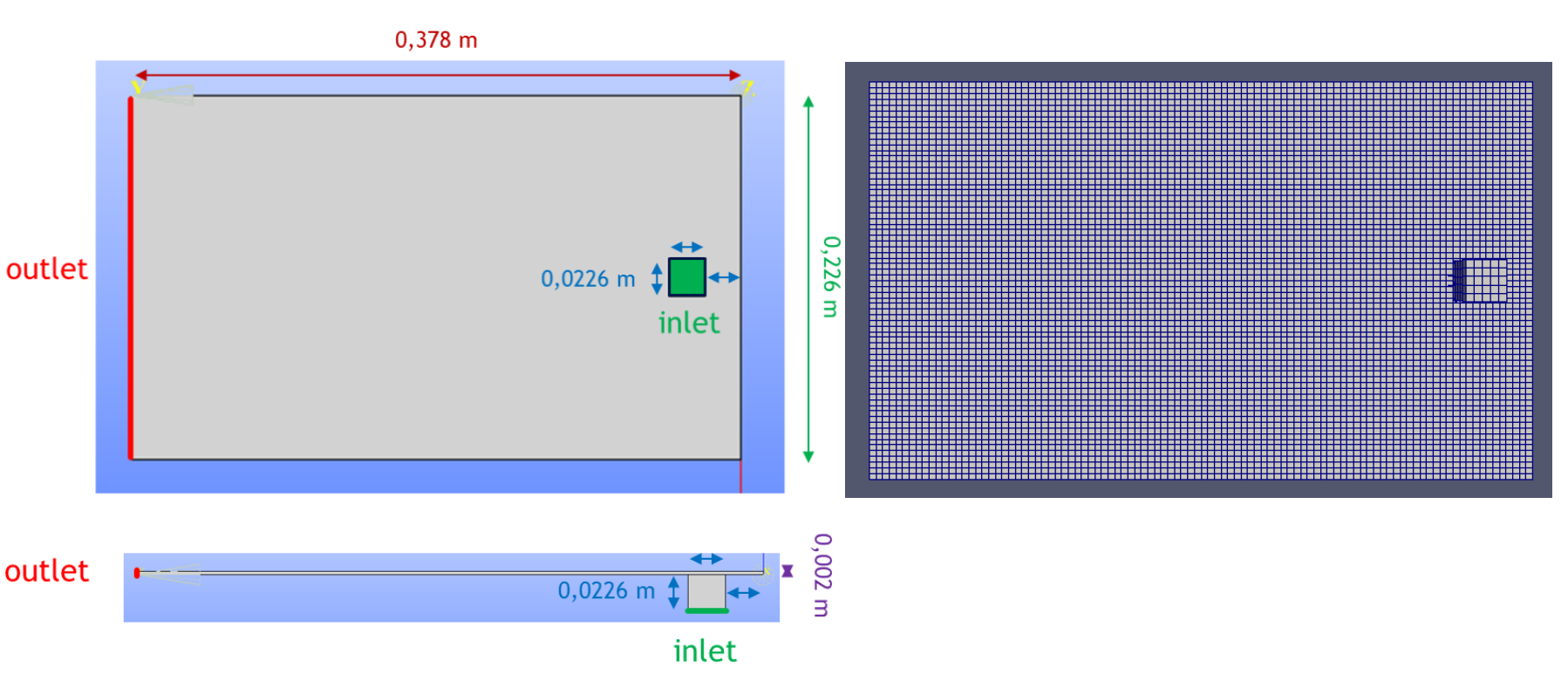
Fig. 3. Bottom view (upper figure) and side view (lower figure) of the simulated geometry (left), meshing of the simulated geometry (right)

The injection is simulated at an isotherm of 453 K, and the value of the parameters of the reactive mix and their origin are detailed on Table 4. The Malkin & Camargo parameters and the coefficient 𝐾_𝜂 values are taken directly from the literature while 𝜌 is taken approximatively from common values of ε₋caprolactam monomer density. 𝜈₀ the kinematic viscosity is obtained with the ratio between the dynamic viscosity calculated with equation at 453 K and the density.

Table 4. Parameters of the reactive mix in the simulation

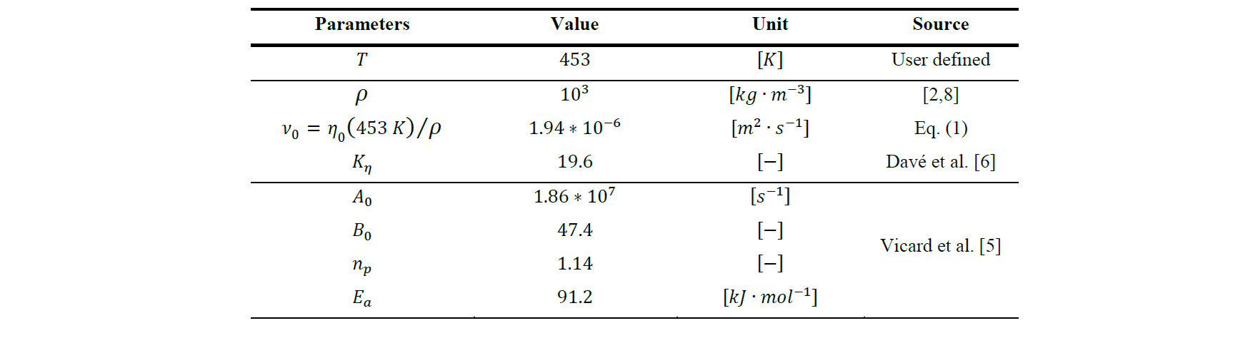
Fig. 4 shows the distribution of the polymerization at t = 40 s of the injection, and at t = 123 s, when the domain is fully filled. At t = 3 s, the resin has started expanding around the inlet which continuously let new resin pass through, hence the distribution of the conversion: the further the resin is from the inlet, the higher its conversion is until it reaches the limit of the domain. At t = 123 s, aside from the outlet, the previous observation does not change. The very low conversion around the inlet shows that the new resin constantly pushes older resin out. The higher conversion value observed further from the inlet means that the polymerization will reach its completion faster at these locations. However, around the middle of the outlet, a zone where the conversion has gone over 0.1 can be observed.

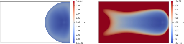Fig. 4. Distribution of the polymerization conversion 𝑎 at t = 40 s (left) and at t = 123 s (right)

Similar observations can be made concerning the distribution of the kinematic viscosity at t = 40 s and at t = 123 s exposed in Fig. 5, but with a sharper transition between high and low viscosity zone. This is expected since the exponential relation between viscosity and polymerization implies that they have the same monotonicity. As such, an isolated high viscosity zone can also be observed near the outlet.

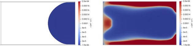
Fig. 5. Distribution of the kinematic viscosity 𝜈 at t = 40 s (left) and at t = 123 s (right)

These observations can be explained with the shape of the flow front and by looking at the flow front. Indeed, the resin flows out of the inlet with a roughly parabolic front, until it reaches an edge. However, the front at t = 40 s shows that its center part will flow until it reaches the outlet. Hence, as the resin is injected, its older parts will be located either at the edge of the domain or at the center of the front. Then, with the progression of the polymerization, the rise of the viscosity becomes exponential and eventually reaches a point where it acts similarly as a solid for the new resin. This is especially showcased by the velocity distribution, shown at t = 123 s in Fig. 6. The direction and the norm of the velocity vectors shows that newly injected resin preferentially flow around high polymerization zone.

Fig. 6. Distributions at t = 123 s of the velocity norm with loosely scaled vectors in the parallelepiped’s median plane

4 Conclusion

In this study, an experimental work on the rheology of the reactive PA6 resin has been presented, which showed the influence of polymerization and crystallization on the dynamic viscosity and led to the establishment of a relation to compute its initial viscosity depending on the temperature. Further investigations will be needed in order to model the influence of polymerization and crystallization on the viscosity.

Then, an injection simulation integrating Camargo’s version of Malkin’s Model in both the transport equations and the dynamic viscosity has been conducted. It has shown the influence the injection has on the age of the resin and how it can affect the flow of the resin through its increasing viscosity.

In future works, the heat transfer equation will be integrated alongside crystallization following a similar procedure. Particular attention will be paid to the integration of Vicard’s version of Hiller coupling. Indeed, this aspect comes with an induction time for the crystallization initiation adding the difficulty of keeping track of the polymerization and the crystallization history of the flow in an Eulerian framework [5]. Then, dual-scale flow simulations using the Darcy penalized Navier₋Stokes equation [14], coupled with the aforementioned reactive flow will be conducted. Numerical benchmarking strategies using analytical, experimental or numerical will be conducted in order to ensure the quality of the simulation procedure. This will allow to have accurate simulation of the reactive resin behavior in term of heat, flow and conversion. Then, these simulations will be confronted to microscale tow information extracted from a real textile specimen [15]. This will permit to evaluate the influence of permeability and double scale porosity in fibrous preforms on the overall polymerization and crystallization of the geometry. At a later stage, an instrumented RTM mold using a mixing head to inject the reactive mix in a glass fibre preform will be used to validate the simulation results.

Acknowledgements

Financial support from the Occitanie Region is acknowledged. The authors wish to thank E. Roussel (ThermoFischer Scientific) for letting us use the Thermo Scientific™ HAAKE™ MARS™ 60 rheometer.