1 Introduction

Surface integrity of machined products and the related mechanical properties define their reliability and functional performance [1]. The most significant surface characteristics such as microstructure, roughness and hardness are strongly influenced by machining process parameters and cooling conditions, especially for components usually made of high strength materials such as titanium alloys [2, 3]. In fact, titanium alloys, and in particular the Ti6Al4V alloy, have an excellent combination of strength, ductility, and high temperature properties [4]. Although the largest user of titanium is still the aerospace industry, nowadays some titanium alloys are employed also in many different fields [5]. In particular, biomedical field is one of the most significant, which is taking advantages of the chemical (i.e. corrosion resistance, biocompatibility) and mechanical properties (i.e. stiffness, density)  of titanium alloys to build artificial implants for worn-out or broken body parts, such as artificial hip-joints, knees and teeth [6, 7].

Another important aspect, which must not be underestimated, is the greater environmental compliance currently required by the modern manufacturing processes to meet the sustainability concept based on the reduction of energy, materials, resources, waste and hazardous substances involved [8]. Critical considerations concerning the use of cutting fluids have been carried out through in depth studies on pros and cons of their employment [9]. The massive use of cutting fluids leads to health problems for workers and it is also harmful to the surrounding environment. For this reason, on the one hand dry machining performance improvement is being tested, and on the other hand alternative solutions such as minimum quantity of lubricant MQL or cryogenic coolant are being applied in metal machining processes [10, 11].

In this context, the influence of machining parameters on the material performance has been evaluated defining and analyzing a mixed-level full factorial design able to evaluate the relationships between the process parameters (cutting speed, feed rate and cooling conditions) and the resulting measured factors namely surface roughness, surface hardness, grain size and wear rate. This paper shows a deep statistical analysis detailing the surface integrity response based on different machining parameters. The overall results permit to clearly define the links within the input and the output variables, identifying different operational conditions for surface integrity improvement and process parameters optimization. Finally, a regression analysis has been performed on the experimental results in order to define the output factors trend considering the process parameters effects.

2 Materials and methods

The workpiece material was Ti6Al4V titanium alloy, in the shape of disks. The experimental tests were performed by varying the process parameters, using the conditions as shown in Table 1. The chemical composition of the initial material is given in Table 2.

Table 1. Experimental tests conditions and parameters.

Table 2. Chemical composition of Ti6Al4V Titanium alloy.

The Ti6Al4V alloy disks were produced from sheets. Each disk had 127 mm of starting diameter and 3 mm of thickness. The machine used was a Mazak QuickTurn 10 CNC turning center, and the orthogonal cutting operation consisted of reducing the diameter of the disk until a maximum value of 80 mm ending diameter. Experiments for the orthogonal tests were setup in such a way to ensure the absence of undesired effects on the machined surface related to transient condition and they were executed as follows.

Firstly, the cutting tool insert was fixed in the tool holder and aligned, and then the disk was mounted in the mandrel held in the chuck of the CNC turning center. Fig. 1 shows the machining process set up. The tool was brought close to the rotating workpiece. Afterwards, the tool enters the workpiece and continues cutting at the prescribed feed rate until the prescribed end-of-cut diameter, and then instantaneously retracts at maximum feed. The utilized cutting tool are coated carbide with an advanced PVD TiAlN coating (Kennametal® grade: KCU10) with triangular shape - TNGG432FS series and mounted on a tool holder (providing rake and clearance angles of 7 ° and 11 °, respectively) and held in a Kistler 9121 three-component piezoelectric dynamometer for cutting force measurement.

The MQL tests were carried out applying to the cutting zone a vegetable oil emulsion by means of an external nozzle to the cutting zone, while the cryogenic coolant (LN2) was applied likewise on the cutting region bringing to a surface temperature of −185 °C. After machining, all samples were sectioned, embedded in mounting resin and subsequentially they were polished and etched, through Kroll acid, in order to perform the metallographic analysis. The microstructural variations such as grain size changes have been evaluated using a scanning electron microscope (SEM).

Five repetitions were performed for the measurements and each test was replicated 3 times. The surface roughness was measured using a Zygo7300® optical white light interferometry-based surface profilometer. The surface and subsurface hardness were measured using a micro hardness indenter Future Tech F-7, starting with an initial hardness of 354 HV_0.05 in the bulk material. Finally, concerning the tool wear, a fresh tool has been used for each experimental test. The flank wear and the crater wear have been evaluated by means of the Zygo7300 ® profilometer, analyzed with its related software MetroPro® comparing the edge radius measured before and after the cutting test. The wear criterion was based on the worked distance to reach the ending diameter from the starting one, hence on the amount of removed material.

Afterwards, a statistical analysis was carried out on the results using the Minitab software, in order to evaluate the influence of the process parameters and cooling conditions on roughness (Ra), surface hardness (HV), grain size (Dim) and tool wear rate (VB) of the examined samples.

Analysis of variance is a collection of statistical models based on the law of total variance, where the observed variance in a particular variable is partitioned into components attributable to different sources of variation, and so it is used to analyze the difference among group means in a sample [12].

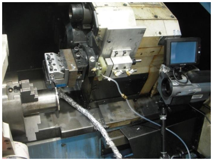
Fig. 1. Tool-workpiece configuration for orthogonal cutting operations.

3 Results

Before carrying out the statistical analysis, assumptions are made. Therefore, if the null hypothesis is true, changing the levels of the factor has no effect on the mean response. Instead, if the null hypothesis is false, the opposite is true. Obviously, as in this case, if there are more different factors the initial hypotheses are directly proportional to the number of variables. The ANOVA partitions the total variability in the sample data into two component parts and the total variability in the data is described by the total sum of squares that can be partitioned into a sum of squares of differences between treatment mean and the grand mean. There is also a partition related to the number of degrees of freedom that corresponds to the sum of squares identity. The ratio between the treatment sum of square and the degrees of freedom is called the mean square for treatment. Then, the values found as shown in the Table 3 need to be used to compare the F-ratio with another F, called F of Fisher (tabulated according to the degrees of freedom and the level of significance), that represent a critic value above which the null hypothesis must be rejected. After this computation, the analysis can be considered complete. As follows, it is also possible to find a P-value for this test statistic.

Table 3. Analysis of variance.

As Fig. 2 shows the analysis of variance for the considered dimensionless factors always exhibited a p-value lower than 0.05, while the p-value of 0 indicates that the factor is significant.

Fig. 2. ANOVA of the different factors.

3.1 Main Effects Plot

A main effects plot is a graph of the means at each level of a factor. Minitab connects with a line the fitted means at each level of the factor. Central points and factorial points are represented by different symbols and a reference line is drawn at the grand mean of the response data. Fig. 3 shows the main effects plot generated by the variation of the above mentioned parameters.

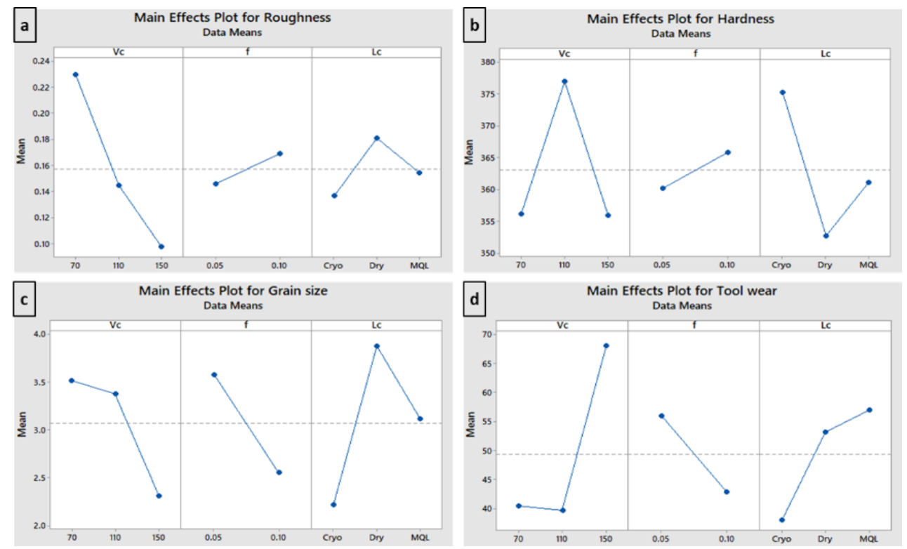Fig. 3. Main effects plot for all the evaluated process inputs and outputs: (a) Roughness, (b) Hardness, (c) Grain size, (d) Tool wear.

From the above graphs, it can be noted how roughness decreases as the cutting speed increases while it boosts with a growing feed rate. Furthermore, it is clear that roughness decreases with increasing lubrication conditions (MQL) and it further decreases under cryogenic cooling conditions. Thus, roughness analysis highlights an improvement trend in surface quality at increasing speed and lubrication and decreasing feed rate. Concerning the surface hardness, the value at the lowest and highest speed is nearly the same, while there is an evident rise at the average speed. Hardness is also directly proportional to the feed rate and to the lubricant/cooling conditions. A different trend occurs for the grain size behavior, in fact there is a slight decrease among the lowest and average speed and then it significantly decreases at maximum speed. Unlike hardness, the grain size is inversely proportional to both the feed rate and the lubricant/cooling conditions. The tool wear decreases with increasing feed rate and in cryogenic cooling conditions, in fact it is known that the coolant at the tool chip interface controls the heat in the cutting zone, rising the tool life and making machining predictable, but tool wear drastically increases at the highest speed.

3.2 Interaction Plots

Interaction plots are useful for judging the presence of interactions; an interaction plot is a plot of means for each level of a factor with the level of a second factor held constant. Interaction is present when the response at a factor level depends upon the levels of other factors. Parallel lines indicate no interaction. The greater the departure of the lines from the parallel state, the higher the degree of interaction. However, the interaction plot does not tell if the interaction is statistically significant. Fig. 4 shows the interaction plots generated for selected case. In the interaction plot for roughness, the lines are almost parallel between speed and feed, especially between the first two speeds; this means that there are no significant interactions between the two. The situation changes slightly in the part relating to speed and lubrication, where between the average and maximum speed there is a significant departure of the lines from the parallel state. In the third part, relating to feed rate and lubrication, there is an evident interaction, it indicates that the relationship between feed rate and roughness depends on the value of lubrication and conversely. The same analysis can be applied to the other graphs, in most of which we notice interactions between all the parameters.

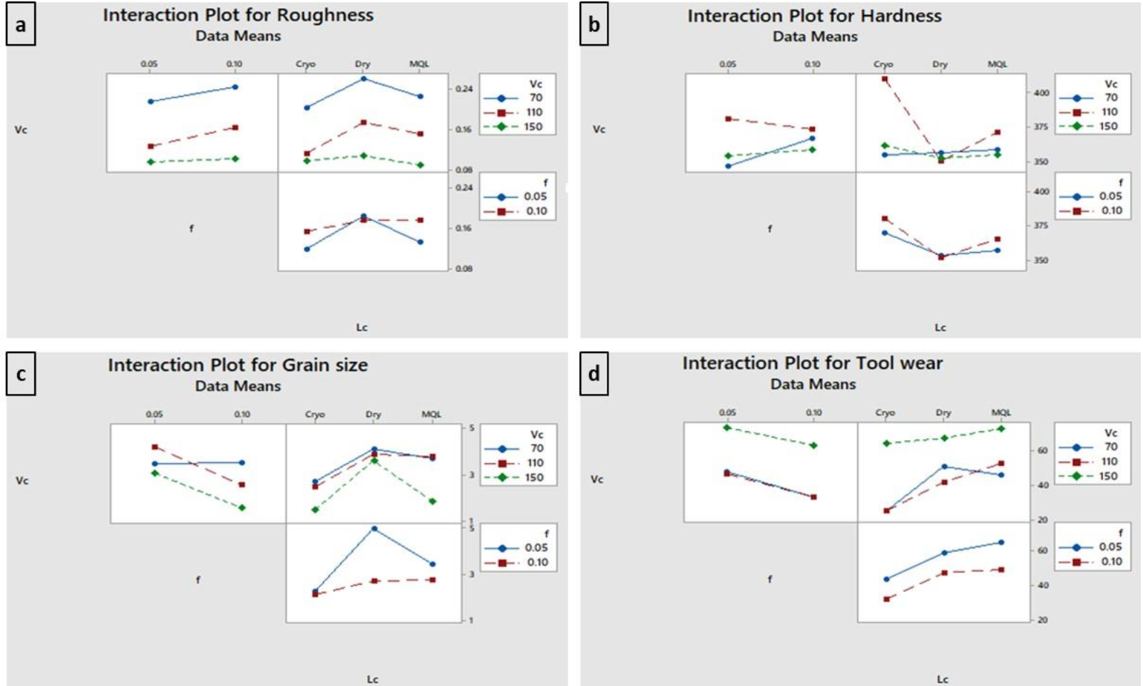Fig. 4. Interaction Plot for: (a) Roughness, (b) Hardness, (c) Grain size, (d) Tool wear.

3.3 Statistical analysis of the experimental results

Concerning the results related to the analysis of variance (ANOVA), the residual plot graphs are shown in Fig. 5, 6, 7, 8 for each measured factor, namely roughness, hardness, grain size and tool wear.

Generally, in the residual plot graph, the first quadrant is the normal probability plot. The points in this plot generally form a straight line if the residuals are normally distributed. If the points on the plot depart from a straight line, the normality assumption may be invalid, but as the number of observations decreases, the probability plot may show substantial variation and nonlinearity even if the residuals are normally distributed.

The second plot should show a random pattern of residuals on both sides of zero. If a point lies far from the majority of points, it may be an outlier.

This condition is directly related to the third plot, the histogram. It has a different distribution from the bell curve if there are a lot of outlier.

Finally, the fourth plot shows all residuals in the order that the data was collected and can be used to find non-random error of time-related effects. If there is a clustering of residuals with the same sign, the correlation is positive. If there are rapid changes in the signs of consecutive residuals, the correlation is negative.

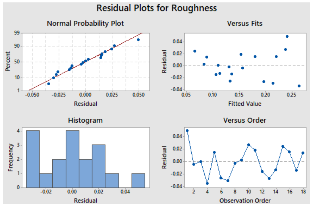Fig. 5. Residual plot for Roughness.

From the analysis of the residual plots, it is possible to see that the normal probability well fit a straight line almost in all the cases; hence, the residuals are normally distributed. In the specific case highlighted for all the factors, there are several outliers, even if not too far from the central line. However, all the trends could be considered linear except for the tool wear where some points depart from a straight line. In fact, the histogram not follow a perfect bell trend.

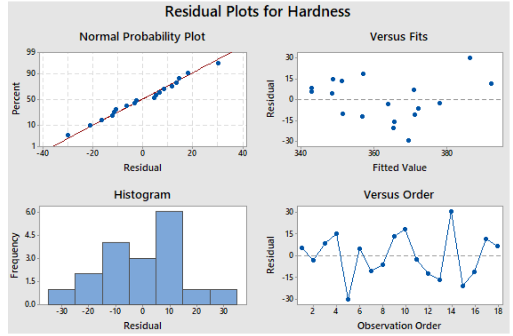Fig. 6. Residual plot for Hardness.

However, the overall statistical results trend might be considered valid. As shown in the fourth quadrant, it could be noticed that there are no cluster of residuals, namely there is a negative correlation, for this reasons the residuals can be treated as an independent of each other.

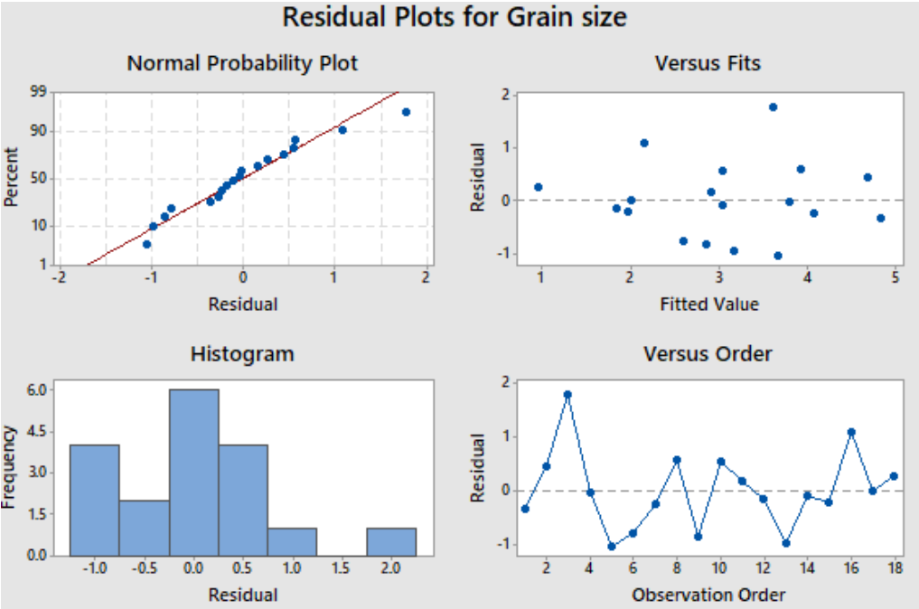Fig. 7. Residual plot for Grain size.

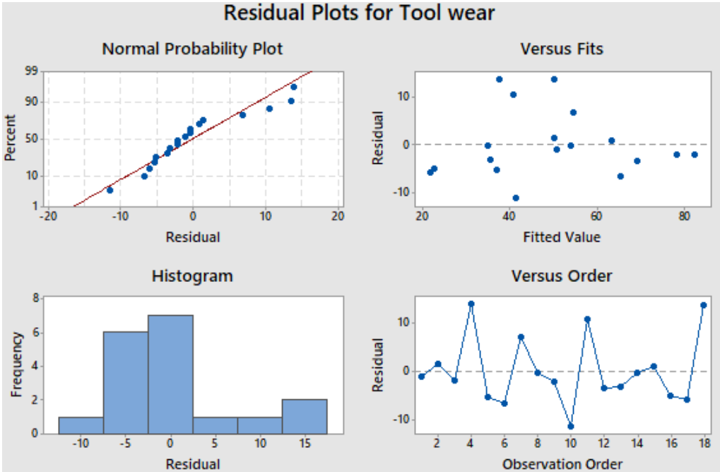Fig. 8. Residual plot for Tool wear.

In order to determine suitable models to describe the output variables trend considering the process parameters effects, after the analysis of variance (ANOVA) a regression analysis was also carried out. The regression equations for each output variables are reported below (Eq. 1, 2, 3, 4).

Surface roughness R_a

Hardness HV

Grain size Dim

Tool wear VB

The above regression equations highlight the set of process parameters that have most influence on each factor, and also with what extent they contribute to the overall measured factor variation. Thus, parameters such as high speed and feed rate have a significant impact on the output factors, as well as the dry and MQL lubricant condition compared to the cryogenic one.

4 Conclusions

This paper presents a deep analysis of the influence of machining process parameters and cooling conditions on the surface integrity of Ti-6Al-4V titanium alloy. In particular, based on the examined experimental data, high speeds led to the best surface roughness although the tool wear increase, while cryogenic conditions preserve the tool wear and increase the surface hardness. Concerning the feed rate, its growth leads to smaller grain size, low tool wear and high hardness but it worsens roughness. Furthermore, it was shown a noticeable interaction between factors, especially among velocity and lubrication conditions.

The regression analysis helps to find the right combinations of parameters to define surface quality improvements. Using the regression equations, it is possible to better specify the effects of the single process parameters on the output variables. For each analysed output factor, the most influencing input parameters are high levels of velocity, greater feed rate and dry or MQL lubricant conditions. Thus, the discussed analysis provides a useful tool to define an operational window for machining Ti-6Al-4V according to the specific requirements.

Acknowledgements

This research was supported by MIUR PRIN 2017 BIONIC.