1 Introduction

Sheet metal typically exhibits an orthotropic behavior related to the rolling process. Such anisotropy material behavior influences the final geometry of deep-drawn parts, stress level prediction in finite element simulations as well as the strain at rupture [1]. Advanced finite element analysis (FEA) continuously adopt anisotropic yield criteria to simulate the forming process and structural behavior of performance-critical components. To amend the accuracy of these forming simulations a huge amount of effort is spent on material parameter identification and experimental validation. In general, parameter identification quality depends on the quantity and quality of experimental test data at hand. Two mechanical approaches exist to acquire this data: homogeneous and heterogeneous tests. The former considers several classical quasi-homogeneous mechanical tests, such as uniaxial tension, simple shear and biaxial tension. These are considered as conventional sheet metal material tests. Practically every conventional test corresponds to a basic specimen geometry that exhibits a specific strain state under monotonic loading conditions. The second approach adopts a more complex specimen geometry to obtain a heterogeneous strain field, wherefrom multiple parameters can be identified simultaneously. The Virtual Fields Method (VFM) [2] and Finite Element Model Updating (FEMU) approaches [3] are currently the main methods to inversely calibrate anisotropic yield criteria from full field data. In the last decade, numerous heterogeneous mechanical tests have been proposed to efficiently extract anisotropic plastic material behavior. Denys et al. [4] proposed a double perforated specimen to enhance the identifiability of a 3D anisotropic yield criterion for thick high strength steel. Coppieters et al. [5] studied the identifiability of the plane stress Hill48 yield criterion via a perforated biaxial tensile specimen. Such designs are mainly based on engineering judgement to increase the sensitivity of the sought parameters. This intuitive approach forms the crux of the problem as the design is user-specific. The latter hampers the industrial application of inverse identification strategies using heterogeneous experiments, recently coined Material Testing 2.0 by Pierron [6]. According to Pierron [6], design and optimization of heterogeneous mechanical tests for the identification of material parameters can be divided in three categories. The first category is based on empirical experience and knowledge by adding hole, slits, or notches, e.g. [4,5]. The second design strategy relies on quantitative evaluation of a heterogeneity indicator with shape optimization, e.g. [7,8,9]. Finally, the third category exploits Topology Optimization (TO) to maximize strain-states and richness of strain fields [10].

This contribution deals with the second category. Souto et al. [7,8] developed an indicator I_T enabling to rank, classify and design mechanical tests considering the level of equivalent plastic strain and strain heterogeneity obtained via a numerical model. A high value of I_T reflects a heterogeneous strain field and this is deemed to enhance the identifiability of the sought anisotropic material parameters. The implicit assumption is that the level of heterogeneity scales with identifiability of the unknown model parameters. Although it is likely that an increase of heterogeneity corresponds with an increase of the sensitivity towards the sought model parameters, it cannot guarantee sufficient identifiability of all model parameters. The latter highly depends on the anisotropic yield criterion under investigation and the actual plastic material behavior. In this paper, the identifiability of the plane stress Hill48 yield criterion via a notched tensile specimen is scrutinized. The paper is organized as follows. First, the shape of the notch is optimized via an I_T-based design strategy. The identifiability of the anisotropic material parameters is then evaluated via the collinearity index and the identifiability index, respectively. Finally, the parameter identification quality of the found heterogeneous specimens are assessed via FEMU using synthetic full field data.

2 Numerical procedure

2.1 Material model

The material investigated here is an industrial cold-rolled steel sheet with a thickness of 1.2 mm. Due to cold-rolling and subsequent plastic deformation, this sheet exhibits anisotropic plastic material behavior as shown by Coppieters et al. [11]. The mechanical properties of the material including the r-values are presented in Table 1. To determine the work hardening properties, standard tensile tests (JIS 13 B-type) were conducted. This data was used to identify the parameters of Swift’s hardening law:

Here, the true equivalent stress 𝜎_𝑒𝑞 is expressed as a power law with K the deformation resistance, 𝜀₀ the initial strain, 𝜀_𝑝𝑙^𝑒𝑞 the true equivalent plastic strain and n the hardening exponent. The identified values are summarized in Table 1 for three orientations: the rolling direction (RD), the transverse direction (TD) and under 45^o with respect to RD (45D). Anisotropic yielding is described by the plane stress Hill48 yield criterion:

The anisotropic parameters can be identified with the aid of the r-values (shown in Table 1) via:

The calibrated Swift law in the RD (see Table 1) is used as reference datum for work hardening implying that equations (3) - (5) are extended with the condition that G+H=1. Solving equation (3) - (5) enables to identify the three anisotropic parameters of the strain-based Hill48-r yield criterion: F= 0.230, H= 0.649, N= 1.412. The latter anisotropic parameters are considered in this study as ground-truth values, i.e. the Hill48-r yield criterion with these reference anisotropic parameters is used to assess the identification quality via FEMU (section 4.3).

Table 1. Swift’s hardening law fitted in a strain range from 𝜀_𝑒𝑞^𝑝𝑙 = 0.002 up to the maximum uniform strain 𝜀_𝑚𝑎𝑥. The reported R-values are measured at an engineering strain 𝜀_𝑒𝑛𝑔 = 0.10 [11].

2.2 Indicator definition and shape optimization process

The shape optimization process driven by I_T is discussed in this section. The indicator I_T [7] is a scalar enabling to quantify the heterogeneity of a mechanical test via the following formula:

The computation comprises five terms, namely the range of the strain state (ε₂/ε₁)_R between the minor (ε₂) and major (ε₁) principal strains, standard deviation of strain state Std(ε₂/ε₁) and of the plastic strain Std(ε_p), ̅ε_Max^p denotes a mean value of maximum equivalent plastic strain- ̅ε ^p at the most relevant strain states(tension, pure shear, uniaxial tension, plane strain tension and uniaxial compression values), and the average deformation- 𝐴𝑣_𝜀̅^𝑝 . Further, W_r and W_a are relative and absolute weighting factors, respectively. Although the relative weighting factors W_r can be adjusted, the factors proposed by Souto et al. [7] are adopted in this study (see Table 2).

Table 2. The absolute weighting factors Wa and relative weighting factors Wr.

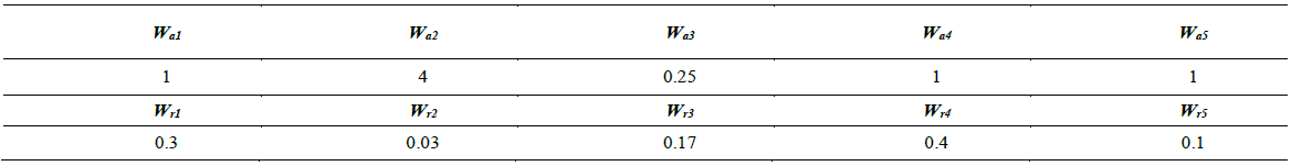
Fig. 1 schematically shows the optimization procedure implemented in a Python script that communicates (i.e. autonomous model generation, meshing, submitting the simulation and post-processing of data) with Abaqus. The optimization process consists of three main building blocks. The first building block is used to determine the critical displacement with the aid of a necking criterion. Once the Python script is launched, two models are created, namely model-0 and model-1 for each iteration. Model-0 consistently imposes an excessive vertical displacement (U2) to determine the maximum allowable imposed elongation of the specimen under investigation. Model-1 then adopts this limitation and is used to extract I_T from the AOI in the second building block. The third building block is the optimization process driven by the Levenberg-Marquardt algorithm to maximize I_T by tuning the parameterized shape of the specimen. The outcome of the third building block is an updated specimen geometry which returns to the first building block for the next iteration. Once the parameter change is marginal, the optimal shape is considered to be found.

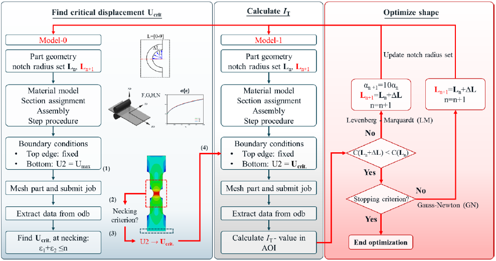Fig. 1 Python Script structure for automatic numerical model, data post-processing and optimization process communicating with Abaqus.

2.3 Optimization problem and FE model

The optimization problem tackled in this paper is relatively simple and based on the concept of a notched tensile specimen to generate a heterogeneous strain field. The resulting heterogeneity obviously depends on the shape of the notch. In order to optimize the shape of the notch via the methodology presented in the previous section, the notch needs to be parameterized. In this work, the notch is parameterized via four coordinates shown in Fig. 2. Fig. 2(a) shows the dimension of specimen and the red shaded area represents the area of interest (AOI). Fig. 2(b) illustrates the enlargement of the notch. The coordinates of A, B, C and D are controlled by the length vector [L_A, L_B, L_C, L_D] and connected via splines. Based on the length vector, the FE model is autonomously created in the first building block of Fig. 1. An example of a generated FE model is shown in Fig. 2(c) including local seed size, element formulation (S4R), boundary conditions and material orientation. The latter dependency is ignored in the present study as the tensile direction was assumed to be aligned with the TD as shown in Fig. 2(c). The length vector [L_A, L_B, L_C, L_D] was subjected to optimization for maximizing I_T in the AOI region.

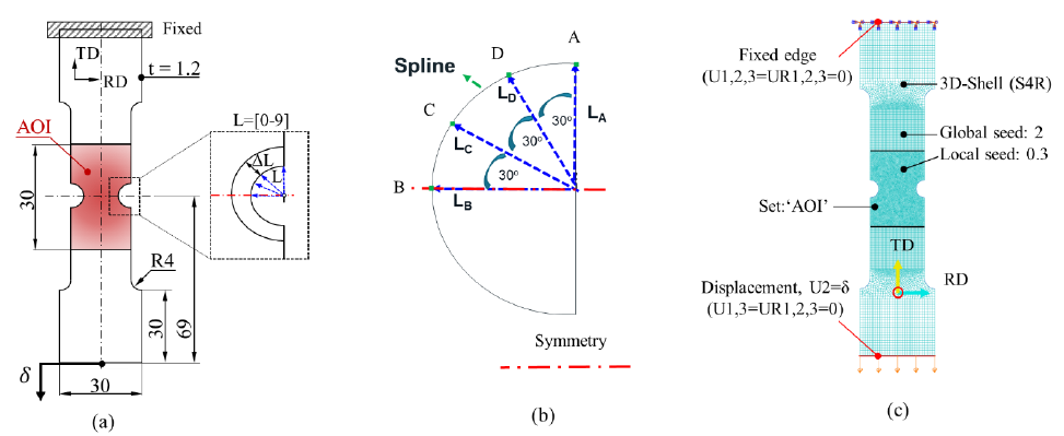
Fig. 2 FE model information with (a) specimen geometry, (b) enlargement part for shape optimization (c) material orientations, mesh information and boundary conditions.

3 Material parameter identifiability analysis

In this paper, the identifiability [12] analysis based on sensitivity of Hill48 parameters is introduced before the FEMU process. In general, sensitivity analysis is defined as a method to assess the influence of optimization parameter variation (geometry, material, loading…) with respect to a numerical response (strain, stress, force…) [13]. The targeted FEMU approach (section 4.3) minimizes the discrepancy with respect to experimentally measured and numerically predicted strain field in the Area of Interest (AOI) of the mechanical test. The discrepancy is expressed by the following cost function:

with n the number of elements in the AOI and θ the vector of unknown anisotropic material parameters. As a consequence, for the identifiability analysis, the required sensitivity matrix 𝑽 is constructed by computing the partial derivative of the strain field with respect to the vector of unknown anisotropic material parameters θ :

with n the number of elements in the AOI and θ the vector of unknown anisotropic material parameters. As a consequence, for the identifiability analysis, the required sensitivity matrix 𝑽 is constructed by computing the partial derivative of the strain field with respect to the vector of unknown anisotropic material parameters θ :

With 𝜺^𝑛𝑢𝑚 generated in strain field and expressed as:

The vector 𝜽 =[𝜃₁, 𝜃₂,…,𝜃_𝑚]^𝑇 is the parameter vector of the Hill48 yield criterion, namely 𝜽 =[𝐹,𝐻,𝑁]^𝑇 with m=3. 𝐕 is thus a (3n × m) matrix evaluated at the reference vector of anisotropic material parameters - 𝜽₀=[0.230,0.649,1.412]^𝑇:

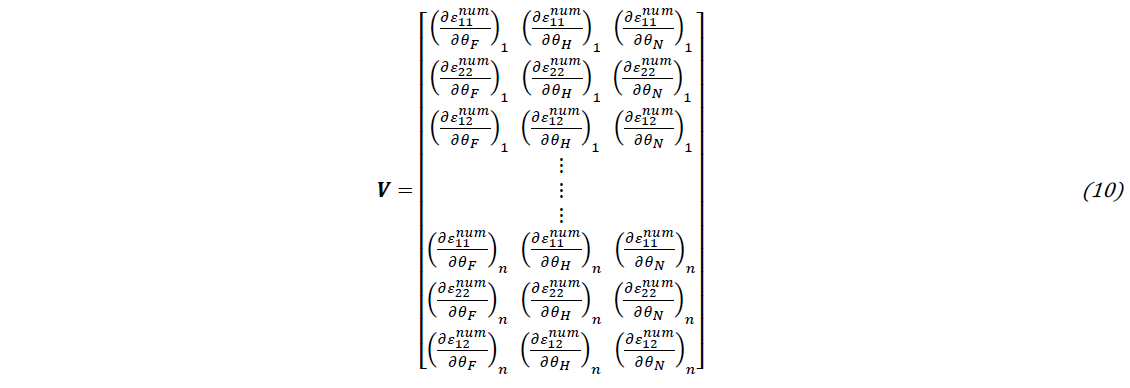
In which (𝜕𝜺_𝑛𝑢𝑚/𝜕𝜃_𝑗)_𝑛 is the partial derivative of the three strain components at element n for certain load step with respect to parameter j in the AOI region. Finite difference approximation was used to calculate the sensitivities adopting the same parameter perturbation value as used in the FEMU process (δ=0.005). To arrive at dimension-free information, the scaled sensitivity matrix S is used:

Here ν_𝑖𝑗 denotes an element of 𝑽, Δ𝜃_𝑗 is an a priori chosen range of reasonable values for 𝜃_𝑗 based on literature or expertise. 𝑆𝐶_𝑖 is a scale factor with the same physical dimension as the corresponding strain component. Finally, to assess the degree of near-linear dependence of the columns of S, the collinearity index [12,14] is calculated. Prior to calculating collinearity, the scaled sensitivities are normalized. This yields the normalized matrix Š_j with the columns defined as:

Where 𝑺_𝒋 is the j^th column in matrix S. This normalization avoids biases caused by differences in the absolute values of the individual sensitivity vectors [15]. The collinearity index is defined as:

Other research [16], however, suggests to assess identifiability via the so called identifiability index:

In both definitions of the collinearity or identifiability index, λ_max and λ_min are the largest and the smallest eigenvalues calculated by Fisher’s matrix H=Š^𝑻Š, respectively. According to Burn et al. [12], a collinearity index of 𝛾_𝑘 > 20 corresponds to poor (high degree of uncertainty) and unstable identification. Gujarati [17], suggested a criterion to discriminate between poor identifiability (I_K > 3), moderate identifiability (2 <I_K < 3) and good identifiability (I_K < 2).

4 Results

4.1 Shape optimization

The outcome of an I_T-calculation depends on the load step at which the strain field is extracted. Indeed, the larger the plastic deformation, the larger the resulting I_T value. This obviously depends on the chosen weighting factors. When adopting the weighting factors shown in Table 2 and applying a simple necking criterion (Fig. 1) to optimize the notch using two different initial guesses for the length vector [L_A, L_B, L_C, L_D] shown in Table 3, the resulting I_T values for Test B and Test C are 0.28 and 0.33, respectively. The final shapes are shown in Fig. 3 along with the generated strain field (plastic equivalent strain-PEEQ). It must be noted that the initial guess strongly determines the optimized shape indicating that local maxima are found. Test A is a regular tensile test having the same width of the homogenous regions of the specimens used in Test B and Test C. When calculating the I_T value for Test A using the framework of Fig.1, a value of 0.25 is found. This is remarkably high compared to the optimized specimens of Test B and Test C. The reason is that the I_T value is calculated in the diffuse neck. This is actually an interesting observation as this suggests that the heterogeneity of the diffuse neck can be exploited to identify the plastic anisotropy. However, further research is required as this observation is likely biased by the choice of the weighting factors as shown in Table 2. When limiting Test A to the uniform strain at 𝜀_𝑒𝑞^{𝑝𝑙 = 0,03} , however, the corresponding I_T value is about 0.01. Given that differential work hardening for the material under investigation (i.e. the anisotropic parameters change as a function of the plastic deformation) stabilizes after about 0.05 equivalent plastic strain [11], the importance of the level of the plastic equivalent strain in I_T can probably lowered when targeting identifiability of plastic anisotropy. In order to have an honest comparison between Test B and Test C, the associated I_T values were calculated for a load step that generate an equal local maximum equivalent plastic strain (approximately 𝜀_𝑒𝑞^𝑝𝑙≈0.5) in both tests. The resulting I_T values are shown in Table 3 (column-Equal Max 𝜀_𝑒𝑞^𝑝𝑙). It can be inferred from Table 3 that Test C is slightly more heterogeneous than Test B.

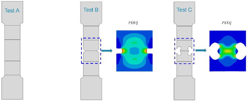
Fig. 3 Geometry of mechanical tests (a) Test A, (b) Test B and numerical strain for PEEQ (c) Test C and numerical strain for PEEQ.

Table 3. I_T value for different initial geometry parameters set and optimal geometry parameters.

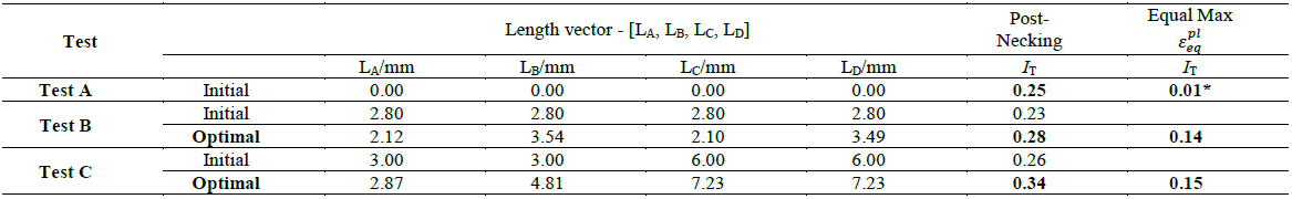
* I_T value at 𝜀_𝑒𝑞^{𝑝𝑙 =0,03} .

4.2 Identifiability analysis

In the previous section, two heterogeneous specimens (Test B and Test C) were found via an IT-based design. The basic research question addressed in this section is whether heterogeneity correlates with the collinearity index and/or the identifiability index of the sought anisotropic parameters. To this end, the identifiability methodology (section 3) is used to evaluate the strain fields generated by the mechanical tests A, B and C. The results are shown in Fig. 4. Fig.4 (a) shows that the I_T value of Test A (I_T = 0.01) is smallest, while Test C is largest (I_T = 0.15) yet very close to Test B (I_T = 0.14). Fig.4 (b) and (c) illustrate the corresponding identifiability and collinearity index of the full parameters set (F, H, N), indicating that both of them are good for Test A, test B and test C. However, both I_K and 𝛾_𝑘 indexes suggest that Test C is best choice. This basically shows that – for the identification problem (i.e. plasticity model and notched specimen) studied here – there is correlation between heterogeneity (measured by I_T) and identifiability (defined as I_K and 𝛾_𝑘). Based on this correlation, it can be stated from a theoretical point of view that Test C will yield the best identification quality when applying FEMU. The latter is scrutinized in the next section.

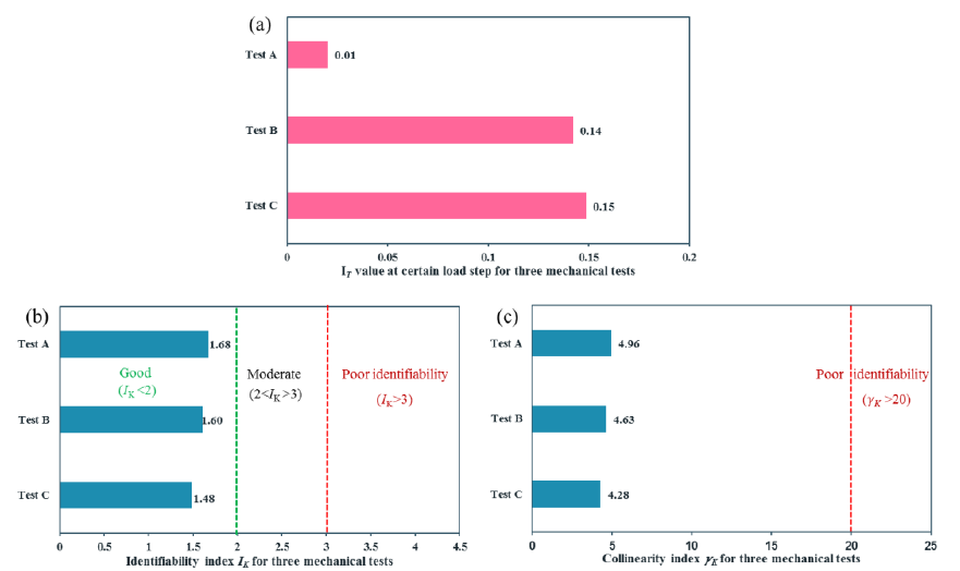Fig. 4 I_T value at certain load step of last increment for numerical simulation (a), corresponding identifiability index using I_K criterion (b) and 𝛾_𝑘 criterion(c) for three mechanical tests.

4.3 Assessment of parameter identification quality via FEMU

The ultimate validation of the I_T-based design is via virtual experimentation and the targeted identification strategy, i.e. FEMU in this study. The virtual experimentation uses a Finite Element (FE) model of the mechanical test with the ground truth material behavior to generate synthetic data which is subjected to identification. The complete measurement chain (including camera calibration, image noise, speckle pattern quality, DIC settings, etc.) can be incorporated by applying an image deformation procedure that uses the generated displacement field from the FE model at the desired load step. Fig. 5 shows the latter process for Test C. The FE mesh is first aligned with an actual speckle pattern (Fig.5 (a)). The node displacements are then used to numerically deform the image (Fig.5 (b)). Finally, the generated image is post-processed with a DIC code to arrive at the synthetic strain field show in (Fig.5 (c)). In this way, all metrological aspects of DIC can be included. Given the large strain gradients and near edge strain localizations in the I_T-based designs (see Fig.3), the approach enables for example to scrutinize the importance of DIC settings in the identification process.

In this study, however, regular DIC settings were adopted yielding a Virtual Strain Gauge of VSG=45 px with an image resolution of 0.039 mm/px. Since the plasticity model used to create the synthetic data is known (the so called reference values shown in Table 4), the identification quality can be directly assessed. The inversely identified anisotropic material parameters for test A, B and C are shown in Table 4. The overall identification quality is assessed by the average relative error R.E.:

with 𝜽^𝑟𝑒𝑓 and 𝜽^𝑖𝑑 the vector of reference anisotropic parameters and 𝜽^𝑖𝑑 (𝜽 =[𝐹,𝐻,𝑁]^𝑇 with k = 3) the vector of inversely identified anisotropic parameters, respectively. It can be inferred from Table 4 that Test A yields the worst identification quality (R.E.= 3.68%). This is not a surprise since Test A is a homogenous tensile test in the TD. Given that in test A the shear stress 𝜎12 in adopted material orientation is zero, it can be expected that the identification quality of the anisotropic parameter N is poor. Table 4 indeed shows that for test A, the parameter N is indeed poorly identified (the R.E. of N is about 4.96%). The identification quality of the test B (R.E.=3.13%) and C (R.E.= 2.49%), which means both of them are clearly better than test A. In addition, Test C yields the lowest R.E. and this is consistent with the identifiability analysis from section 4.2. Finally, the identified yield loci are shown in Fig. 6 along with the reference yield locus. It can be inferred that Test C indeed yields the best identification.

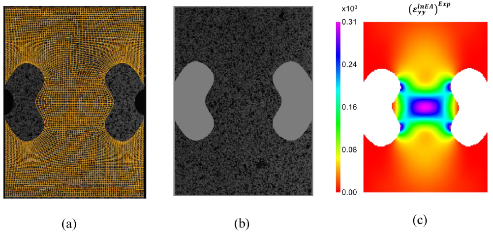Fig. 5. Virtual experimentation: FE mesh projection (a), synthetic image deformation (b) and synthetic strain field after DIC (c).

Table 4. Comparison of correct parameters values and identified parameters values for Test A, Test B and Test C, respectively.

Fig. 6. Normalized identified yield loci compared with the reference yield locus. Test A (a), Test B (b) and Test C (c).

5 Conclusion

This paper scrutinizes the independent validation of I_T-based design of notched tensile specimens for the identification of anisotropic material parameters. The parameterized notch is optimized based on the heterogeneity indicator-I_T . Independent validation is pursued via the identifiability method and parameter identification quality obtained through FEMU using synthetic experimental data. The identifiability method is based on the FEMU cost function formulation and the associated parameter perturbation value. For the studied identification problem (notched tensile specimen and the plane stress Hill48 yield criterion), correlation between the heterogeneity indicator-I_T, the identifiability method and identification quality through FEMU is found. This basically means that – for the studied anisotropic yield criterion – an I_T-based design definitely improves the parameter identifiability. Despite this correlation, however, it cannot be claimed that the presented I_T-based designs are optimal for the problem at hand as heterogeneity is maximized instead of identifiability. In that sense, future research will investigate whether the observed correlation holds true for more complex anisotropic yield criteria. In that regard, the I_T-based design could probably be enhanced by adjusting the weight factors in I_T formulation tailored for identifying anisotropic yield criteria. It must also be noted that the I_T-based designs in this study are disconnected from the material orientation. Given that the identifiability method enables to directly assess the identification quality of the anisotropic material parameters based on a particular strain field, future research will embark on combining I_T and the identifiability method for designing heterogeneous specimens with optimized identifiability towards a subset of anisotropic material parameters. Moreover, the identifiability method will be used to enhance the efficiency of the FEMU approach by a priori determining the identifiable anisotropic parameters. Indeed, the identifiability method enables to determine non-identifiable anisotropic material parameters (e.g. the mechanical test is insensitive to certain anisotropic material parameters or material model is over-parametrized) prior to start the FEMU process.

Acknowledgements

Thanks to financial support from the program of China Scholarships Council (No.201806460097) and acknowledge MatchID for the use of software.