1 Introduction

The mechanical behaviour of sheet metals is usually sensitive to strain, strain rate and temperature. Recently, due to the growth of heat-assisted manufacturing processes [1], strain rate and temperature effects have gained more impact. Hence, accurately predicting sheet metals’ mechanical behaviour, under a wide range of strain rates and temperatures, is increasingly relevant to advance manufacturing processes. To predict such behaviour, thermoelastoviscoplastic constitutive models, characterised by their nonlinearity and a large number of material parameters, can be applied. However, the traditional calibration of such models requires an extensive database with tests performed at a broad range of strain rates and temperatures [2].

The use of full-field measurement techniques, heterogeneous mechanical tests, and inverse methods has reduced the required experimental tests [3]. Applying full-field measurements techniques, such as digital image correlation (DIC), the entire displacement fields at the specimen’s surface can be recorded and directly used to calibrate a constitutive model. The information obtained from these tests can be further enriched using temperature measurements. The constitutive model material parameters can be identified using inverse methods, such as the finite element model updating (FEMU) [4].

Solely using full-field measurements with inverse methods does not guarantee that suitable material parameters are found. An automatic strategy using optimisation algorithms is required to find these material parameters. However, most studies related to constitutive models’ calibration tend to overlook the importance of optimisation algorithms by resorting to familiar ones, such as gradient-based least-squares algorithms [5]. These algorithms may perform well and be suitable for nonlinear least-squares problems, such as the ones formulated using the mentioned inverse methods but may also present disadvantages. A few studies have explored the use of other optimisation algorithms and strategies, such as direct-search and stochastic methods [6–8].

This paper aims to implement different optimisation algorithms in the calibration of a thermoelastoviscoplastic constitutive model. Three heterogeneous thermomechanical tests performed at different average strain rates are used in this work. The FEMU is used as the inverse method, and three optimisation algorithms are applied in the optimisation procedure. The results obtained with different optimisations algorithms are compared in terms of efficiency and robustness.

2 Methodology

2.1 Heterogeneous thermomechanical test

Simulation data from three heterogeneous thermomechanical tests is used as a reference to represent experimental data [9]. Nonetheless, this reference data is based on tests performed on a Gleeble 3500 thermomechanical simulator, using a hydraulic servo system able to impose tension or compression forces, as well as a direct resistance heating system [10]. A uniaxial tension loading is imposed on the specimen, with a heterogeneous temperature field. Finally, the tests are performed at different average strain rates of 10^-2, 10^-3, and 10^-4 s^-1. The temperature field is imposed through the direct resistance heating system, controlling and maintaining the temperature at the specimen’s centre during the test. The specimen’s remaining part presents a temperature gradient due to the machine’s grips’ water-cooling system. The added value of this procedure is the temperature gradient triggering a heterogeneous deformation, providing information on the material’s mechanical behaviour for different temperatures and strain rates.

The reference data is generated by a finite element model of the tests, whose configuration is presented in Fig. 1. For simplicity, the finite element model is restricted only to the region of interest (ROI), defined by a width of 28 mm and length of 60 mm. The finite element model is two-dimensional, assuming a plane stress formulation. Abaqus/Standard [11] software is used in the finite element analysis, and the four-node bilinear plane stress quadrilateral element CPS4 is used, with a large strain formulation. The finite element mesh is composed of 1680 elements. Displacement-driven boundary conditions are imposed on the finite element model’s extremities, at −30 and 30 mm of the reference coordinate 𝑥 (origin at the specimen’s centre).

Fig. 1. Schematic representation of the specimen used in the heterogeneous thermomechanical tests (dimensions in mm). The grips are represented on the extremities of the specimen and the region of interest (ROI) defined for the finite element model [9].

The temperature field acquired with Gleeble equipment usually presents a parabolic shape, symmetrical about the specimen’s centre. Measurements of three thermocouples placed at −40, 0 and 40 mm of the reference coordinate 𝑥, confirm the approximate symmetrical and parabolic shape of the profile along the specimen’s length. Temperature variations along the width of the specimen are neglected. Additionally, it was confirmed that the temperature field remained constant throughout the deformation process [9]. Because of its parabolic shape, each test’s temperature field can be described by a second-order polynomial, as presented in Fig. 2, between −30 and 30 mm of the reference coordinate 𝑥. For the three tests, the maximum temperature of approximately 500 ºC is reached at the specimen’s centre, decreasing to around 360 ºC at −30 and 30 mm of the reference coordinate 𝑥. Therefore, the temperature field is imposed in the finite element model through the second-order polynomial, and the nodes’ temperatures remain constant throughout the test.

The Johnson-Cook thermoelastoviscoplastic constitutive model is adopted [11]. The model is characterised by a multiplicative formulation, decomposing the flow stress evolution in three terms: strain hardening, temperature and strain rate. It can be written as

where 𝜀̅^p is the equivalent plastic strain and 𝜀̅͘^p the equivalent plastic strain rate. The first term describes the strain hardening effect, modelled by the material parameters 𝐴, 𝐵, and 𝑛. The temperature effect is modelled by the temperature 𝑇, the transition temperature 𝑇_tr, governing the threshold of temperature effect, the melting temperature 𝑇_m, and the exponent 𝑚. Lastly, the strain rate sensitivity is modelled by the material parameters 𝐶 and 𝜀̇₀ , defining the threshold of strain rate dependence.

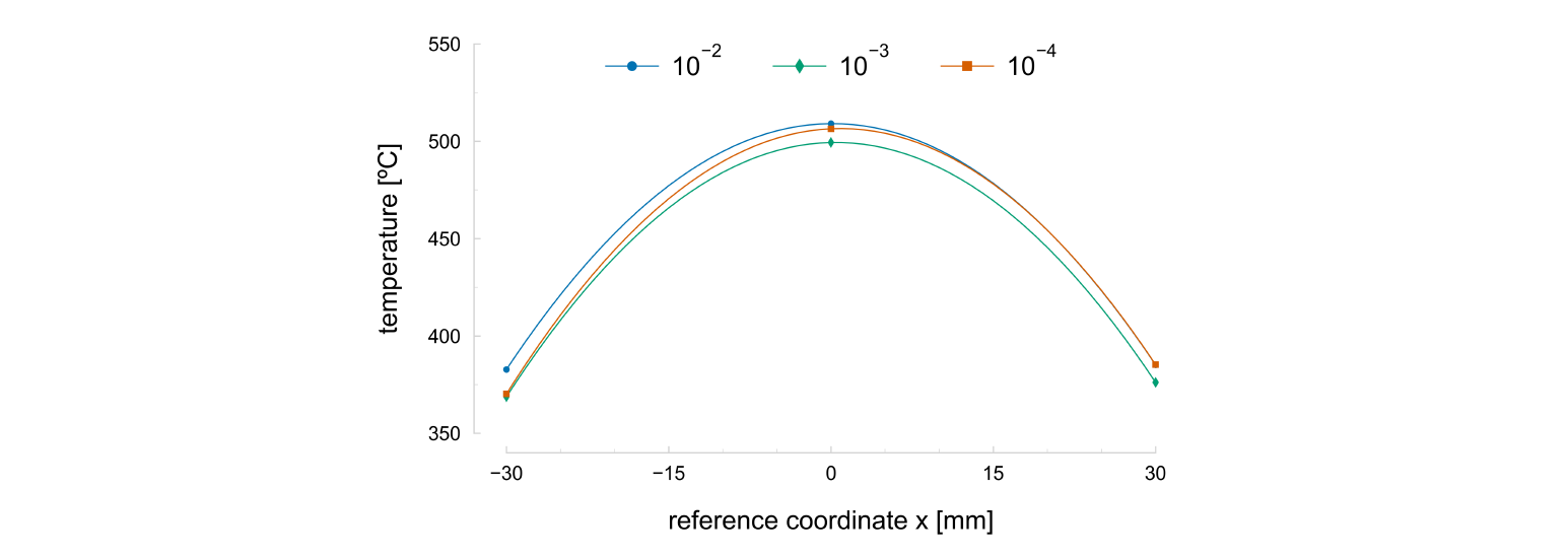
Fig. 2. Longitudinal temperature field of heterogeneous thermomechanical specimen’s longitudinal temperature field described by second-order polynomials. Each curve is identified from the average strain rate of each test (in s^-1).

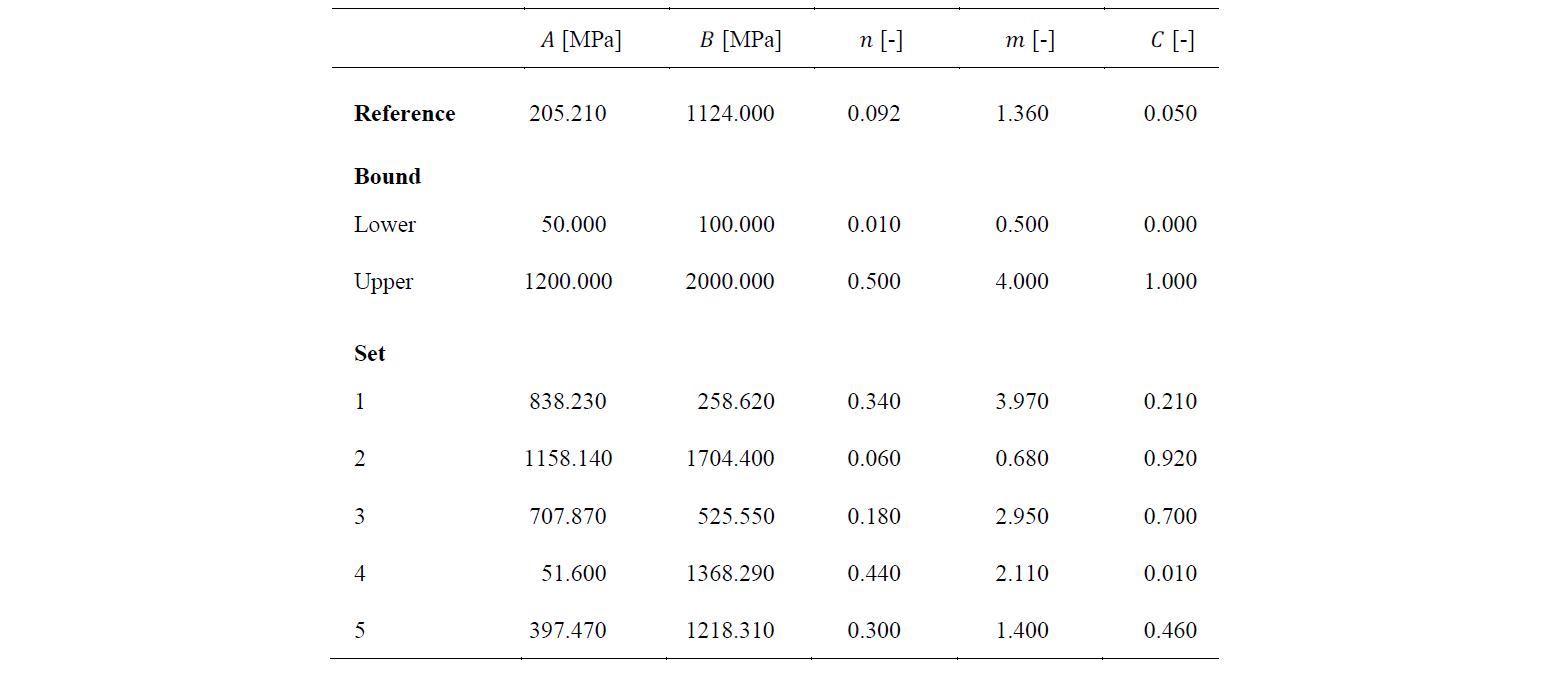
The reference data is created using a set of reference parameters [9], characteristic of a DP980 dual-phase steel (see Table 1). The material is considered isotropic, and the Hooke’s law is used to describe the elastic behaviour, and the von Mises yield criterion is adopted. The elastic properties of the material, namely Young’s modulus 𝐸 = 210 GPa and Poisson’s ratio 𝜈 = 0.30, are known a priori and assumed to be constant in the temperature range of study.

Table 1. Reference set of parameters used in the Johnson-Cook thermoelastoviscoplastic constitutive model to generate the reference data used for calibration [9].

Then, the reference data is generated using the temperature field and the reference set of parameters. This reference data is composed of the displacement field of the ROI (longitudinal and transversal displacements) and the load for each time instant. The reference load for the tests performed at three different average strain rates is presented in Fig. 3. A different number of time instants composes the tests’ reference data, specifically, 47, 58, and 62, respectively, for tests with an average strain rate of 10^-2, 10^-3, and 10^-4 s^-1. It can be observed that the load is sensitive to the average strain rate, as an increase leads to higher values of maximum load.

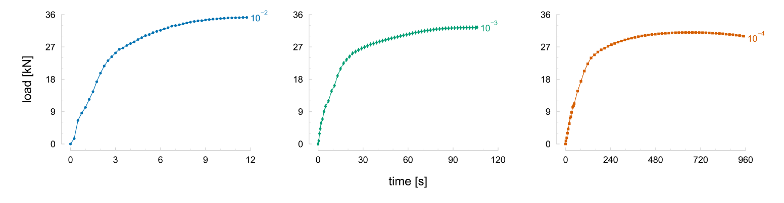
Fig. 3. Load evolution throughout the deformation process of the heterogeneous thermomechanical tests performed at an average strain rate of 10^-2 (left), 10^-3 (centre), and 10^-4 s^-1 (right).

2.2 Finite Element Model Updating

The finite element model updating (FEMU) is used to calibrate the constitutive model. This method is based on the simple idea of iteratively adjusting the finite element model’s unknown material parameters to minimise the difference between experimental and numerical results. The FEMU has been largely adopted in many different applications, partly because of its ease of implementation and flexibility. The objective function to be minimised can be composed of different data, such as strain, displacement and load signal. This flexibility has contributed to an increase in the number of formulations presented in the literature. Recently, the FEMU is mainly being used in combination with full-field measurements. In that regard, the adopted objective function can be written as

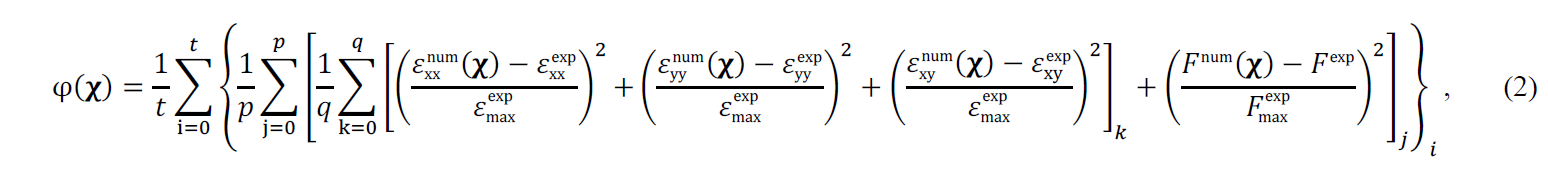
where 𝛘 = (𝐴, 𝐵, 𝑛, 𝑚, 𝐶) is the vector of optimisation variables. The variables 𝑡, 𝑝, and 𝑞 are the number of tests, time instants, and in-plane measurement points. To distinguish between experimental (reference) and numerical variables, the superscripts “exp” and “num” are used, respectively. The variable 𝜀_max^exp represents the maximum strain value of all in-plane components and time instants for each test. Analogously, 𝐹_max^exp represents the maximum load value of all time instants for each test. Because the displacement field represents the raw data, the strain field is computed from the displacement field using a total Lagrangian formulation. The reference strain field is computed before the calibration procedure, and the updated strain field is computed after every finite element simulation, from the extracted numerical displacement field.

2.3 Optimisation

The optimisation procedure controls the FEMU method and is performed by different algorithms. The optimisation procedure is implemented in Python programming language, using the optimisation algorithms from the SciPy library [13]. This library has several optimisation algorithms (e.g., gradient-based, stochastic), providing the user with easy implementation in its programs. Three optimisation algorithms of different types were selected for the optimisation procedure: Levenberg-Marquardt, Nelder-Mead and Differential Evolution algorithms.

The Levenberg-Marquardt (LM) is a gradient-based algorithm that uses the approximated Hessian and Jacobian matrices [14]. It used to calibrate constitutive models [15–17] because it is well suited for solving nonlinear least-squares problems. The LM algorithm requires the user to select an initial solution, and if not well chosen, it can lead to convergence difficulties or to finding local minima, instead of the global minimum. Nonetheless, if the problem is well-conditioned and a suitable initial solution is selected, the algorithm can rapidly converge.

The Nelder-Mead (NM) algorithm is one of the best known and simpler direct-search algorithms used in unconstrained optimisation [18]. The NM algorithm uses a simplex that begins with a set of points for every optimisation variable plus one, considered its vertices. Based on a series of transformations of the simplex, the algorithm iteratively reduces the simplex size. The algorithm is known to achieve satisfactory results in few iterations but may also present convergence problems. Comparatively to gradient-based algorithms, this algorithm stands out for not requiring the use of derivatives.

The Differential Evolution (DE) is a population-based stochastic algorithm that generates new solutions from other solutions [19]. The DE algorithm can be characterised by its ease of implementation, robustness, and finding the global minimum of a problem in most attempts. However, a significant drawback of DE is its high computational cost and low convergence rate compared to other optimisation algorithms. On the other hand, when compared to other population-based stochastic algorithms, DE tends to overperform them. As it is common in population-based algorithms, the number of solutions used as the population can significantly impact the convergence and success of the optimisation procedure [20]. Moreover, the DE algorithm requires the definition of variables bounds to generate the initial set of solutions, either manually, randomly or distributed over the search space.

Contrary to the DE, the LM and NM algorithms are suitable for unconstrained problems. However, to limit the three algorithms’ search space, lower and upper bounds are defined for the variables (see Table 2). The defined bounds are based on the order of magnitude of each variable, and special attention was taken not to restrict the search space overly. On the DE algorithm, the bounds are directly imposed, while for LM and NM algorithms, a transformation of the variables is used. For all the algorithms, the optimisation variables are normalised by its bounds. Considering 𝑥̂_i = 𝑥_i.⁄𝑥₀) the variable 𝑥_i normalised relative to its initial value 𝑥₀, the lower and upper bounds, 𝑥_i^min and 𝑥_i^max, are normalised as

where 𝑥̂_i^min and 𝑥̂_i^max are the normalised bounds. Then, the transformed variable 𝑋̂_i for 𝑥̂_i ≥ 1 corresponds to

and for 𝑥̂_i < 1 corresponds to

Using these transformations guarantees that the algorithms achieve feasible solutions, i.e., solutions lying inside the search space.

3 Results

The material parameters 𝐴, 𝐵, 𝑛, 𝑚, and 𝐶 are defined as the optimisation variables to identify. The melting temperature 𝑇_m, the transition temperature 𝑇_tr, and the parameter 𝜀̇₀ are considered known a priori and kept fixed throughout the optimisation procedure. These parameters are kept fixed because the first two have specific physical meaning, and the third may increase the problem of non-uniqueness of the solution [21].

To mimic image noise from actual full-field measurements, random noise from a normal Gaussian distribution is added to the reference data’s displacement field, while the load signals are kept noiseless. To evaluate the robustness of the methodology and performance of algorithms, three data sets are used as reference data for the calibration: (i) without noise; (ii) with noise of amplitude 10^-5 mm; and (iii) with noise of amplitude 10^-3 mm. The objective function values using the variables reference set are 0.0, 3.130 × 10^-9, and 3.017 × 10^-5, respectively, for each data set.

Because the LM and NM algorithms are sensitive to the initial solution, five different initial sets are generated using the Latin hyperspace sampling method, generating solutions evenly distributed over the search space (see Table 2). The number of initial sets was arbitrarily selected as equal to the number of optimisation variables. This sampling method does not consider the reference set, avoiding an initial bias towards the global minimum. The distribution of the variables of each generated initial set over the search space is shown in Fig 4. These five initial sets are used for the LM and NM algorithms, while for the DE algorithm, a population of 50 solutions is generated using the same sampling method. This population size was chosen as ten times the number of optimisation variables.

Table 2. Reference set and upper and lower bound of optimisation variables. The sets of optimisation variables represent the initial sets used for the Levenberg-Marquardt (LM) and Nelder-Mead (NM) algorithms.

The three algorithms are, in general, used with the default settings defined in the SciPy library. The exception is the step size for the finite difference approximation of the Jacobian in the LM algorithm, set equal to 10^-3. The adaptive setting in the NM algorithm is also set, enabling the algorithm to adapt its parameters to the problem’s dimensionality.

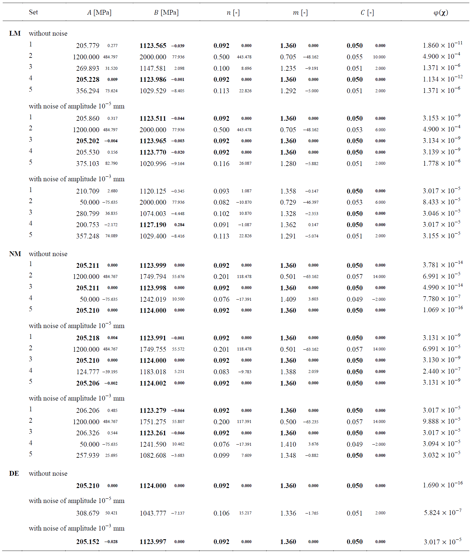
The final solutions and objective function values obtained in the optimisation procedures are summarised in Table 3, for the three algorithms. Additionally, in Fig. 5, the objective function’s evolution throughout the function evaluations is represented for the three algorithms.

Considering that for final solutions within 0.1% of error from the reference solution, the algorithms achieve the global minimum, it is observed that the LM algorithm presents the worst performance of the three algorithms. Overall, the LM achieves the global minimum only twice, whereas the NM algorithm achieves the global minimum six times, and the DE algorithm can find the global minimum in two out of three attempts. The fact that LM cannot achieve the global minimum more often can be related to the step size for the finite difference approximation of the Jacobian, which is probably not small enough. The algorithm could benefit from starting a new optimisation procedure, using the obtained solution as the optimisation’s initial solution, and reducing the step size.

LM and NM algorithms’ results confirm their sensitivity to the initial set, with results varying depending on the initial set. This is particularly evident when the variable 𝐴 of the initial set is close to its upper bound, as it is the case of set 2. In this situation, the solution stagnates very early, either in the upper and lower bound of variable 𝐴. Based on these results, it can be said that avoiding initial solutions close to the variables’ bounds can potentially decrease the chance of the algorithm converging there. In general, variables 𝑛, 𝑚, and 𝐶 present higher success rates in achieving the reference solution. However, set 5 with the LM algorithm shows local minima, which are very susceptible to this algorithm.

The effect of noise in the results is quite interesting, as it is observed that noise can benefit the algorithm. In the case of the LM and NM algorithms, the final solutions achieved are, in general, very similar between the data sets without noise and with noise of amplitude 10^-5 mm. However, in the LM with initial set 3, it is observed that the presence of noise benefits the algorithm in achieving a better solution than without noise. When the level of noise is increased to an amplitude of 10^-3 mm, both the LM and NM algorithms are not as efficient in achieving the reference solution, but the NM algorithm appears to be less negatively affected by the presence of additional noise. The DE algorithm appears to be less affected by noise regarding the final solution, as each variable solution of the data set with noise of amplitude 10^-3 mm is within 0.1% of error from the reference solution. However, the final solution for the data set with noise of amplitude 10^-5 mm is not close to the reference one, but it can be related to a local minimum. To further investigate the effect of noise in the DE algorithm, more attempts should be performed, as the DE algorithm is not deterministic, and a component of randomness always exists. The objective function convergence is also affected by the presence of noise. For example, for the LM algorithm with the initial set 1, where the final solutions are relatively similar, the algorithm converges around 1000, 600, and 50 function evaluations, respectively, for data sets without noise, with noise of amplitude 10^-5 and 10^-3 mm.

In summary, the differences between the LM and NM algorithms are more evident in terms of convergence rate, where the first tends to converge rapidly, whereas the former typically requires a higher number of function evaluations. A single attempt was performed for the DE algorithm with each data set, and it appears to be more robust than the other two algorithms. Nonetheless, it generally requires a high number of function evaluations to converge to the global optimum. Considering the use of multiple initial sets for the LM and NM algorithms, it can be considered a good substitute to the DE algorithm.

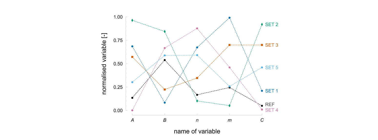
Fig. 4. Distribution in the search space of the optimisation variables, normalised by its bounds, in each initial set for the Levenberg-Marquardt (LM) and Nelder-Mead (NM) algorithms. The reference set is also represented.

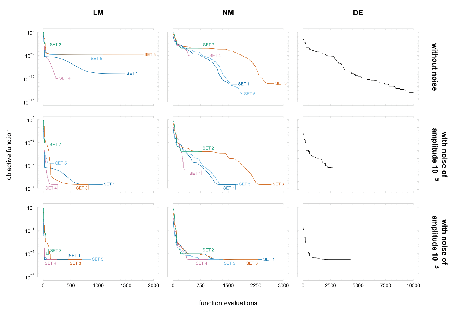
Fig. 5. Evolution of objective function throughout function evaluations using the Levenberg-Marquardt (LM), Nelder-Mead (NM), and Differential Evolution (DE) algorithms, represented from left to right. Results correspond to data sets without noise, with noise of amplitudes 10^-5, and 10^-3, from top to bottom.

4 Conclusion

A methodology to calibrate thermoelastoviscoplastic constitutive models based on full-field measurements and the FEMU is considered to reduce the number of thermomechanical tests involved. Three heterogeneous thermomechanical tests performed at different average strain rates are used as reference data required by the calibration procedure. By taking advantage of a modern programming language library, three optimisation algorithms are easily implemented in the calibration process, namely the Levenberg-Marquardt (LM), Nelder-Mead (NM), and Differential Evolution (DE) algorithms. The algorithm’s results are compared for three data sets, involving different noise levels introduced in the reference data’s displacement field. The DE algorithm demonstrates the most robust algorithm by reaching or being very close to the global minimum in two out of the three data sets. However, it is also susceptible to local minima even though less than the LM and NM algorithms. Moreover, the number of function evaluations required for convergence by the DE algorithm is higher than the others. A strategy using multiple initial sets could be used to circumvent the sensitivity of LM and NM algorithms to initial sets. Additionally, it would be interesting to explore the use of the DE algorithm early on to reduce the search space, and then use LM or NM algorithms to fine-tune the solution. Nonetheless, this approach could be susceptible to local minima in the vicinities of the global optimum. In the scope of the present work, a calibration software was developed in Python programming language, which will allow the easy implementation and combination of optimisation algorithms.

Table 3. Final solutions and objective function values obtained in the optimisation procedure using the Levenberg-Marquardt (LM), Nelder-Mead (NM) and Differential Evolution (DE) algorithms. Results correspond to data sets without noise, with noise of amplitude 10^-5, and 10^-3 mm. The smaller font size values represent the relative error (%) of each variable’s final value to the reference one. The values in bold indicate that the error to is smaller than 0.1%.

Acknowledgements

This project has received funding from the Research Fund for Coal and Steel under grant agreement No 888153. The authors also gratefully acknowledge the financial support of the Portuguese Foundation for Science and Technology (FCT) under the projects PTDC/EME-APL/29713/2017, PTDC/EME-EME/31243/2017 and PTDC/EME-EME/30592/2017 by UE/FEDER through the programs CENTRO 2020 and COMPETE 2020, and UID/EMS/00481/2013-FCT under CENTRO-01-0145-FEDER- 022083. The authors also would like to acknowledge the Région Bretagne for its financial support and BPI France under project EXPRESSo. M.G. Oliveira and J.M.P. Martins are, respectively, grateful to the FCT for the PhD grants SFRH/BD/143665/2019 and SFRH/BD/117432/2016.