1 Introduction
This work addresses the use of machine learning algorithms to enhance the performances of the Proper Generalized Decomposition (PGD) model reduction techniques. In fact, PGD uses a fixed-point iterative algorithm to build a reduced basis “a priori” without any previous knowledge of the solution. The employed rank-one update greedy algorithm requires the solution of several lower-dimensional problems.
Within the PGD rationale, the solution of a 3D problem defined in a plate or shell geometry reduces to the solution of a series of 2D and 1D problems. Thus, the unknown field (e.g., 3D displacement, temperature, …) is assumed expressed as a finite sum of products of functions, one depending on the in-plane coordinates (x,y) and the other depending on the through-the-thickness coordinate (z).
This separated representation was applied in our former works in a diversity of physics: (i) elastic and inelastic problems defined in plate, shell and beam-like geometries, including dynamics, contact, plasticity, damage, fracture, … [1-5]; (ii) thermal models defined in plates and laminates [6-7]; (iii) flows of Newtonian and non-Newtonian fluids in thin flat and rough gaps [8-12]; (iv) electromagnetism in stratified composites [13]; … These formulations, in principle intrusive with respect to their use in existing commercial software, were successfully formulated for reducing intrusiveness [14-17]. The present paper constitutes a step forward.
First, several 3D solutions are used to train a neural network for extracting, under the stringent real-time constraint, the optimal out-of-plane function from which to enrich the usual coarse-grained description (e.g. 2D shell) to recover all the needed richness (3D) while keeping the computational complexity the one characteristic of 2D simulations. Of course, this through-the-thickness enrichment depends on some local and global information that must be efficiently learned, justifying the use of deep learning, among the existing regression techniques. For illustrating the just described procedure, in that follows, we address the solution of a heat problem involving 3D effects in a thin domain involving a 2D discretization.
2 Methods
2.1 Problem statement
The steady state heat conduction problem will be solved in a thin square plate of width a=1m and height h=0.1m. Thus, the in-plane coordinate x=(x,y) takes values in (0,a)x(0,a), with the out-of-plane coordinate (z) taking values in (0,h). The thin plate lateral surfaces will be insulated, while the temperature u(x,y,z) is prescribed on the top and bottom surfaces, with a constant temperature on the last, and linearly evolving on the former. In particular, u(x,y,z=0)=U and u(x,y,z=h)=350y+50 (all the units being in the metric system).
The steady heat conduction problem is solved in that plate domain, with a source term “q” (internal heat generation) and a constant thermal conductivity K. The training was performed by assuming different values of the temperature prescribed on the bottom surface (U), as well as the value of the source term (q) and the conductivity (K), with U taking values in the interval (0,400), q in the interval (0,2000) and K in (0.01,0.1).
A rich enough DoE is defined and the resulting heat problems solved for the chosen values of the parameters (U,q,K) by using the in-plane-out-of-plane PGD solver. A large number of the computed solutions is used for training the neural network whereas the remaining calculation are reserved for testing the constructed model (regression) accuracy.
2.2 High-fidelity 3D solver
The temperature field is expressed as
that introduced into the problem weak form, and solving the in-plane and out-of-plane resulting 2D and 1D problem, allows computing both functions involved in equation (1) related to each i-mode of the finite sum, following the usual PGD rationale, widely considered in our works previously referred.
2.3 Extracting the through-the-thickness behavior
Now, if the in-plane domain is equipped with a 2D mesh, at each node of that mesh the solution reads
that once normalized, represents a valuable way to express the solution evolution throughout the domain thickness.
2.4 2D approximation
Usual finite element -FE- approximations defined in the in-plane domain, with the index k referring to the different nodes of the 2D mesh, reads
2.5 Enriched 2D discretization
Now, by injecting the approximation (3) into the steady state heat problem weak form, and after integrating on the domain thickness, it results a fully 2D with as unknowns the nodal coefficients alpha in Eq. (3).
The most critical point when modelling and the solving the resulting 2D problem by using the approximation (3) is the choice of the normalized enrichment function at each node of the 2D mesh discretizing the in-plane domain (functions f(z) in Eq. (3)).
2.6 Machine learning based training
A shallow neural network is trained from the solutions given by (2) for each parametric choice (U,q,K) in table 1.
Table 1. Set of parameters values used to train the neural network
The set of solutions generated using the parameters grouped in Table 1, is divided in three sets (training, validation and testing set). A new set of problems with the parameters given in Table 2 is used to avoid overfitting.
Table 2. Set of parameters for obtaining an additional dataset for testing purposes
The through-of-thickness function extracted at each node from the computed solutions exhibits an almost parabolic shape and thus can be approximated accurately with a second-degree polynomial, with a maximum error of 2.7%.
The trained regression vanilla type feedforward multilayer perceptron consists of an input layer, one hidden layer and an output layer. The input layer nodes are the variables required to describe the problem and specify the location of the node where the function is to be predicted. Since the top surface temperature varies only along the y-coordinate, the shape of the generic functions does not change along the x-coordinate and thus, only the y-coordinate of the in-plane node will be included in the neural network input parameters list.
Thus, the input neurons are selected to be: (i) the node y-coordinate; (ii) the internal heat generation q; (iii) the material conductivity K; (iv) the temperature prescribed at the bottom surface temperature U; and (v) the temperature on top surface at location (y-coordinate) of the considered node.
3 Results
After obtaining the 1D generic functions using the neural network, the 2D finite element model can be easily solved for calculating the in-plane function, and then reconstruing the fully 3D solution from a single and simple 2D solution.
The solutions for all problems defined in Table 2 are computed and each of them compared with the reference PGD solution. To compare both solutions, the error at each node is computed, and from them the error norms and the mean relative error, for each problem, with the maximum resulting values grouped in Table 3.
Table 3. Error of the enriched 2D formulation
The resulting error, with a maximum mean error of 0.36%, is very satisfactory compared to the computational gain. Solving the problem using PGD would require the computation of multiple enrichment terms while iterating between the in-plane function and the out of plane function for each term, within a fixed-point iterative algorithm. In the proposed method a simple 2D calculation suffices for computing a very detailed 3D solution, with a very high accuracy as soon as the through-the-thickness function is well chosen.
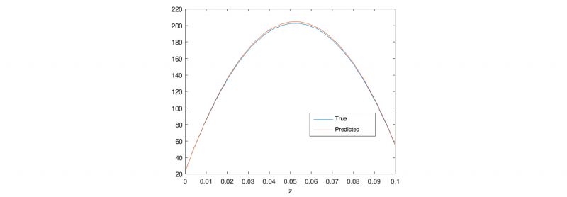
Concerning those through-the-thickness functions, Table 4 reports the mean and maximum residuals, with the one with maximum gap depicted in Figure 1.
Table 4. Error in the predicted through-the-thickness functions
Fig. 1. Predicter versus reference though-the-thickness function exhibiting the largest gap
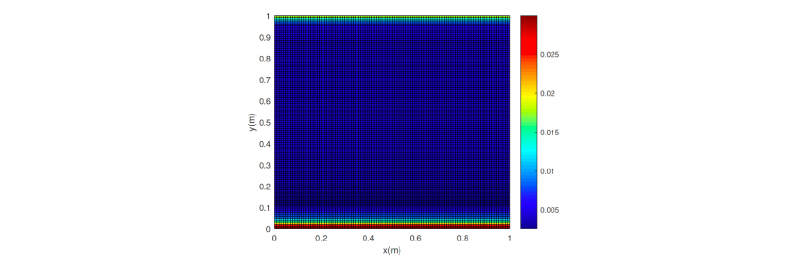
Figure 2 plots of the maximum error at each node of the in-plane discretization for the solution exhibiting the maximum error, where a very small error of 2.99% occurs in the vicinity of the border y=0.
Fig. 2. Error space distribution
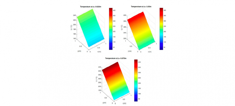
The solution related to the maximum mean error, is depicted in Figure 3 at different z-coordinates to illustrate the reconstruction of the fully 3D solution.
Fig. 3. Solution at different heights (z-coordinate)
4 Conclusions
In the present work authors illustrate an appealing approach of combining artificial intelligence and model order reduction. The proposed technique enhances the performance of the PGD model reduction technique in the sense that a fully 3D solution is obtained from a single 2D calculation. For that purpose, a through-the-thickness function is provided by a trained Neural Network, from high fidelity solutions obtained by using the in-plane-out-of-plane PGD-based separated representations.


