1 Introduction

Induction hardening is one of the most surface heat treatment processes widely employed in aerospace and automotive industries [1,2] to improve material performance by changing mechanical properties of the critical zones [3]. The process consists of two steps; an electrically conducting component is first heated by electromagnetic induction to a temperature within or above the transformation range and then cooled by an immediate quenching. This process has the advantage of providing a very short surface heat-up times, a precise control of the treated zone, a good fatigue performance, and a good reproducibility [4]. However, the control of mechanical parts quality goes through the prediction and the optimization of the induction hardening process. The main difficulty behind this optimization is the multi-physics property of induction hardening (electromagnetism, thermal, metallurgical, and mechanical field) in addition to the large number of process parameters; thanks to advanced numerical simulation tools, modelling and solving physical problems is possible by using some conventional discretization methods such as finite element, finite volume, etc. Nevertheless, passing through those methods to optimize multi-physics parametrized problems is often regarded as a key issue. In fact, when the number of parameters increases, the multi-query simulation approach becomes inefficient and makes optimization procedure very time consuming and computationally expensive. In order to alleviate such issues, reduced order modeling (ROM) techniques constitute an appealing alternative to standard discretization techniques given the interesting compromise in terms of computational cost, speed of execution, and results accuracy. Among these ROM techniques, which require in most cases the knowledge of equations describing the physics, Proper Orthogonal Decomposition (POD) [5], reduced basis methods [6], and Proper Generalized Decomposition (PGD) [7] have been widely used. However, some new strategies were developed to compute the parametric-based solution from sampled data, collected from experimental measurements or from finite element simulations, such as Sparse Subspace Learning (SSL) [8] and sparse Proper Generalized Decomposition (sPGD) [9].

The aim of this work is to investigate the possibility of applying a new approach based on the ROM to compute the temperature evolution in a gear under the effect of induction heating process parameters in almost real-time. To achieve this goal, the POD based reduced-order model was used and then followed by artificial intelligence (AI) techniques for regression purpose. It is worth pointing out that the proposed approach relies only on data and doesn’t require any knowledge of the full-order formulation or modification of the numerical finite element (FE) codes, hence the approximated parametric solution is constructed by using a datadriven non-intrusive ROM approach.

Based on a set of precomputed solutions of the full-order FE models (called snapshots), collected at some sparse points in the space domain and for different values of input parameters, the POD enables to build a reduced basis onto which the initial FE solution could be projected. The reduced state vector of the snapshots data, so-called POD modal coefficients, were then considered and multiple regression methods were used to fit the low dimensional POD modal coefficients. In other words, the POD modal coefficients represent the approximated solution of the ROM.

The rest of the paper is organized as follows: Section 2 defines the methodology and the numerical technologies with more details. Section 3 defines the process and the data generation. The results are then presented in Section 4 and Section 5 concludes this work.

2 Dimensionality reduction by POD and regression methods

Consider a set of P snapshots Ti = T(t, μ_i)_i=1,…,P ∈ ℝ^N, computed by solving the full-order FE model at each time step and for different values of input parameters µ_i, where t, µ = (µ₁,…,µ_S), and N are the time, the set of S parameters, and the dimension of the FE solution, respectively. The snapshot matrix M ∈ ℝ^NxP is defined such that M = [T₁ T₂ T_p] and each column contains a snapshot. To find the reduced basis, the singular value decomposition (SVD) is applied to M as follows:

where U ∈ ℝ^NxN and V ∈ ℝ^PxP are orthogonal matrices containing the left and right singular vectors of M, respectively. Σ ∈ ℝ^NxP is a rectangular diagonal matrix containing the singular values σ_k of M sorted in a decreasing order. The reduced POD basis, B = [ϕ₁, ϕ₂, …, ϕ_R], is defined as the first R left singular vectors of M (i.e. first R columns of U) corresponding to the R largest POD singular values. Thus, singular values provide a quantitative guidance for choosing the size of the POD basis. In practice, POD provides an efficient representation of the snapshot data in low-dimensional subspace of dimension R, much lower than N, such that

where ϕ_j and α_ji are called POD modes and POD modal coefficients, respectively. In matrix form, B ∈ ℝ^NxR and a_i = B^T.T_i where a_i ∈ ℝ^R .

Now, instead of using P snapshots T_{i, i=1,…,P} of dimension N to fit the model to the data, the low-dimensional representation of the initial snapshots a_{i, i=1,…,P} will be considered. Then, the return back to the original space could be achieved using Equation (2). The literature review illustrates that many regression techniques can be used to approximate the POD model coefficients for any choice of parameters included in the vector µ, such as sPGD which is based on the separated representation approach and enables quite rich approximations for high dimensional problems in a low-data limits [10], multiple linear regression [11], support vector regression SVR [12], random forests [13], and gradient boosting [14]. These techniques will be applied in the current work.

Let now consider a database, composed by P combinations of input parameters µ_i and their corresponding response a_i. The response matrix is written as A=[u₁, …, u_R] where each row of A contains a vector a_i. Regression techniques consist in defining, in different ways, the approximated function f_k as follows:

where ε_k is the residual term. The origin of regression error may depend on physical issues or the choice of hyperparameters associated to each method.

3 Problem statement and data generation

Induction heating (IH) is becoming one of the preferred heating technologies in many industrial applications [15] due to its advantages regarding fast heating, efficiency, accurate control, and cleanness compared to other classical heating techniques. Basically, it consists in applying an alternating current (AC) to a copper coil surrounding a conducting workpiece, a magnetic field generated by the AC induces an eddy current and consequently a heating by Joule effect of the workpiece (see Fig.1). In addition, IH combines multiple physics and it can be modeled by several FE codes, in which partial differential equations (PDE) describing electromagnetic and thermal problems are solved. Equations governing the physics at hand are not presented in this paper, more detailed information can be found in [16]. In order to optimize and improve IH performances applied to a spur gear of 22 teeth (studied workpiece shown in Fig. 2), multiple parameters can be taken into consideration such as process, material, and geometrical parameters. However, as a first step of this study, three important parameters were considered while the other ones were kept constant. The selected parameters and their lower and upper limits are shown in Tables 1.

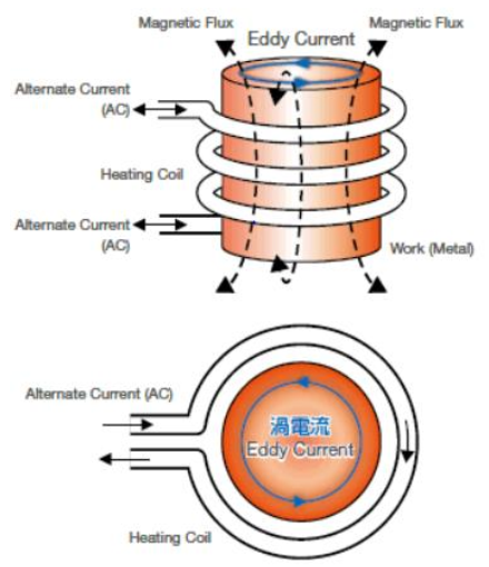Fig. 1. Principle of induction heating [17]

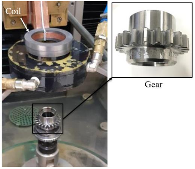Fig. 2. Experimental set-up of the induction heating.

Table 1. Input parameters and their lower and upper limits.

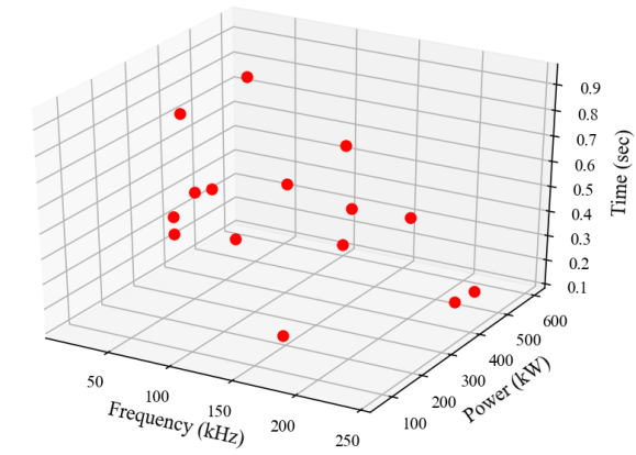
As mentioned before, dimensionality reduction requires a set of precomputed high-fidelity solutions, collected by solving the original full-order model for different values of input parameters. For this reason, the commercial finite element software FORGE® was used. It is worth mentioning that the model has two symmetry planes and hence only half-tooth of gear is modeled for enhancing the computational efficiency. Besides, several FE simulations were conducted using Latin Hypercube Sampling (LHS) of experiments [18]. Particularly, it guarantees a good coverage of each parameter space. According to the LHS, a total of 15 simulations have been generated. as shown in Fig. 3. Therefore, it is worth seeing how well the regression methods perform with small amount of data.

Fig. 3. Latin Hypercube Sampling

The post-processing of the temperature evolution was done at 14 specific points representing the main heat-affected zones as shown in Fig. 4.

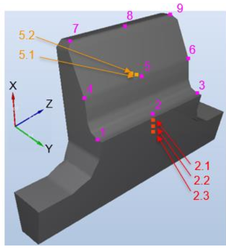Fig. 4. Measurement points.

4 Results and discussion

It is worth pointing out that the above-mentioned simulations result in different process times and consequently different dimensions. To alleviate such issue, a normalization of the discrete times was done for each simulation as follows:

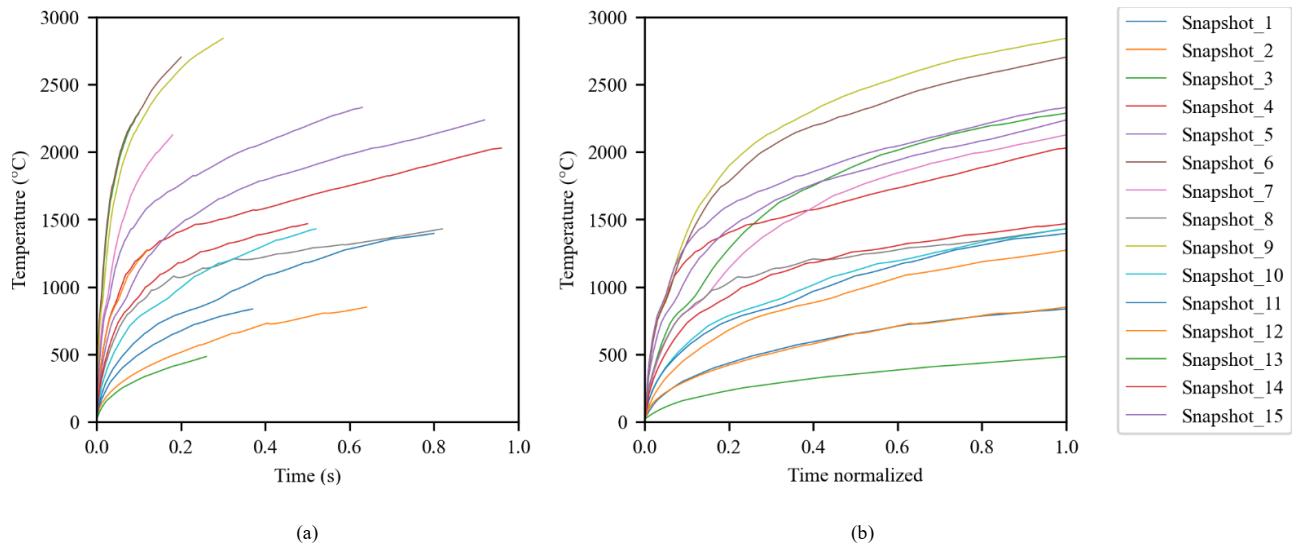Fig. 5. Temperature evolution at point #1 based on (a) the reel time, (b) the normalized time.

A snapshot matrix was defined for each measurement point, then the POD modes and their corresponding modal coefficients are computed as explained in Section 2. The left singular vectors of the snapshot matrices were truncated to the first singular vector which correspond to the POD mode. This choice is made in accordance with the fact that, with the first singular value, more than 90% of the variance is retained as shown in Fig. 6. It is worth pointing out that only results for points (#1, #5, #9, and #2.3) were shown in this section for the sake of clarity.

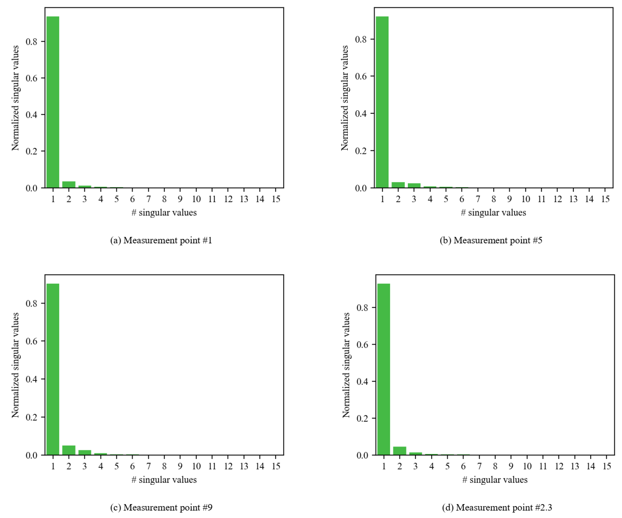Fig. 6. Normalized singular values of the thermal field for 4 snapshot matrices.

After computing the modal coefficients, a surrogate model for each one of them and for each measurement point was constructed. Before that, the standardization of the input parameters was applied to avoid problems related to units and different scaled features, then the dataset was divided into training and testing subsets (80% of data is used to build the models and 20% to evaluate their accuracy).

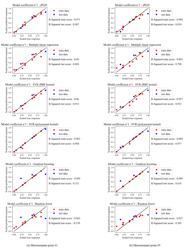
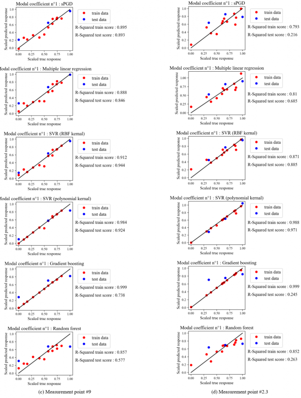
Fig. 7. shows the scaled real versus the scaled predicted values of modal coefficients for points (#1, #5, #9, and #2.3) using different regression methods implemented in python packages except the sPGD. The red points correspond to the data used to build the regression model and the blue ones correspond to the testing data used to evaluate its accuracy. When points are too close to the black line, the surrogate model provides a good fit to data. Indeed, the dispersion of these points with respect to the black line gives a visual indicator of error. Additionally, the score associated to each regression model for the red and blue points was also presented in Fig.7. It is clear that the results are slightly different from one measurement point to another and the SVR regression model provides the best fit followed by the sPGD, then the other techniques.

Fig. 7. Scaled predicted versus scaled real response for 4 measurement points.

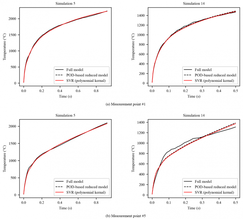
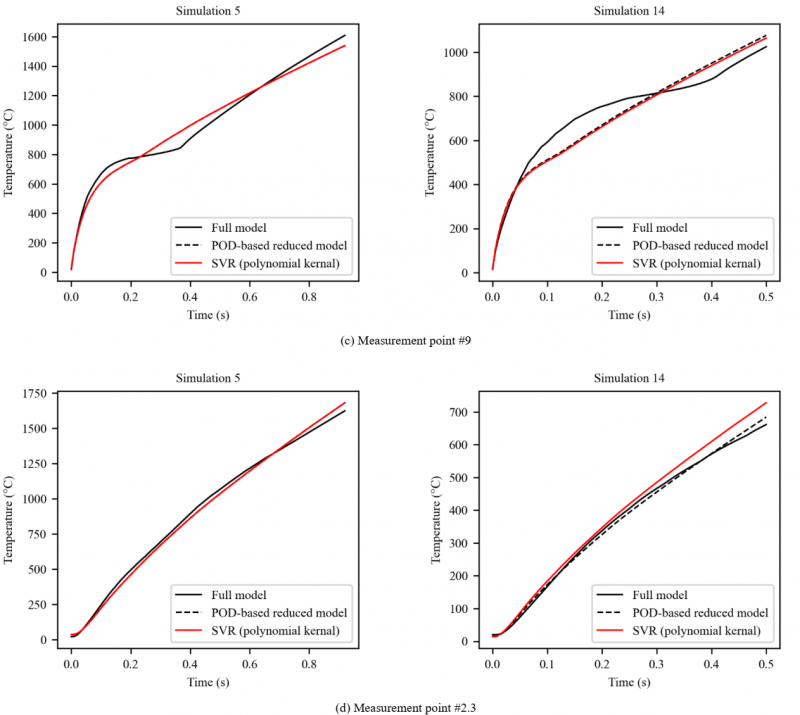
Fig. 8. shows the temporal evolution of the temperature obtained by the full model, the POD-based reduced model (i.e. Using equation (2) with real values of modal coefficients), and the SVR regression model (i.e. using equation (2) with the predicted values of model coefficients) which provides comparatively the best fit.

It is worth mentioning that the curves of the SVR regression model (red curves) should overlap the dashed black curves which is almost perfectly done for both the training (left data) and testing data (right data) and for the four measurement points as well. For point #2.3, a slight difference between the red and black dashed curves of the test data was obtained. However, this error is still acceptable, and the predicted and the real curves show the same trend. Nevertheless, since one POD mode and consequently one model coefficient as a response for the regression was considered, it seems that it is not sufficient to describe in a proper way the real temporal evolution of temperature. To improve the approximation accuracy, two modes and modal coefficients were considered instead of one, but the obtained results of regression were not good enough and leading to a problem of overfitting, despite the optimization of the hyperparameters associated to regression techniques. This part constitutes a work in progress.

Fig. 8. Comparison of the temporal evolution of temperature between the initial full model, the POD-based reduced model (with the real values of model coefficients), and the SVR regression model (with the predicted values of model coefficients) for 4 measurement points: data used for creating the regression model (left) and data used to evaluate the regression model accuracy (right).

5 Conclusion

In this paper, an approach, based on dimensionality reduction by POD coupled with regression techniques to fit a model to the POD modal coefficients, was proposed to compute the temperature evolution during the multi-physics parametric-based induction heating process in low-data limit. The approach was successfully applied for 14 sparse measurement points in the space domain, in which a basis with a single vector was built and consequently a single POD modal coefficient was computed and used for creating the surrogate model. A good approximation was provided, and a quite good performance of some regression techniques was shown as well. A comparative investigation showed that the SVR regression model gives the best fit to the data.

Nevertheless, regression methods work well with the first POD modal coefficient associated to the first POD mode, but this latter doesn’t fit perfectly the initial FE solution. Applying regression methods to the second and third modal coefficients do not provide good results. Future developments are required in order to improve the accuracy of the approximated solution. Once a better approximation is obtained, the solution will be extended to address the whole space domain using interpolation techniques.

Acknowledgements

This work was conducted with the help of the French Technological Research Institute for Materials, Metallurgy and Processes (IRT M2P). The authors would like to acknowledge IRT- M2P and the partners of the project TRANSFUGE led by IRT M2P.