1 Introduction

Vast improvements of light-weight structures to reach weight-savings in transportation industries originate from the ubiquitous scientific, economical and societal demand to reduce the fossil-fuel consumption and cost as well as to decrease the emission of green-house gases [1]. Driven by the weight-saving benefits when combining unique physical and mechanical characteristics of different metallic alloys, manifold combination of similar and dissimilar materials are joined. The efficient joining of similar or dissimilar materials via solid-state joining processes can enable weight-savings, since various combinations of similar or dissimilar metallic alloys that are widely used for manufacturing of large-scale structures in automotive and aerospace industries, can be welded. In particular, through the refill Friction Stir Spot Welding (refill FSSW) process, numerous solidification problems such as pores and cracks are avoided and high-quality joining of materials that are even considered as “unweldable” are enabled. The refill FSSW process was developed and patented by Helmholtz-Zentrum Geesthacht (HZG) [2,3] and many different material combinations in similar [4,5] and dissimilar joint configurations, such as Al/Mg [6,7], Al/steel [8,9] and Al/Ti [10,11], were already welded.

Conduction of regression analyses with machine learning algorithms to build predictive models based on data can be a powerful and efficient alternative in comparison to calibrating and validating analytical models or numerical high-fidelity models. In the fields of materials mechanics, the application of machine learning and data mining approaches has been reviewed in [12] to discuss various examples on the identification and utilization of relationships along the process-structure-property-performance chain, enabling further understanding of underlying physical mechanisms. For classical programming, specific rules are explicitly defined on input-data processing to produce desired answers, whereas for machine learning algorithms, answers are trained to be related to input-data through learning of necessary rules. Consequently, when those rules are identified via machine learning algorithms, applied to new data, the resulting answers can be new and original [13].

Yamin et al. [14] investigated the refill FSSW process to identify relationships between process parameters and the cross tensile strength (CTS) for similar aluminum alloys. Based on a Box-Behnken Design of Experiments (DoE), statistical analysis and the response surface methodology were used to establish an analytical model for the prediction of CTS. An interpretation on how the different process parameters influence the CTS was provided, which was only based on linear regression. The aim of this study is to expand this perspective via the deployment of non-linear prediction models. Therefore, different non-linear machine learning algorithms are used to build an accurate predictive model to foresee the CTS of refill FSSW AA7075-T6 joints. For further improvement of the joining process, it was targeted to build a prediction model with lower prediction errors than the commonly used analytical model based on linear regression. In order to evaluate and select the most accurate model, a comparison of the different employed algorithm is drawn and an interpretation is provided.

2 Refill Friction Stir Spot Welding

In the solid-state joining process of refill FSSW, a non-consumable tool composed of two rotating parts is utilized in combination with a probe and a sleeve, as well as a stationary clamping ring to join two or more similar or dissimilar materials in lap configuration. Two variants of the process can be implemented, depending on the plunging part of the tool being the sleeve or the probe. The most used variant is the sleeve plunge process variant, where, initially, the to-be-joint materials are clamped against a backing anvil via a clamping ring whereas sleeve and probe start to rotate uni-directionally. Translational movement is executed on the rotating sleeve and probe move in opposing directions. Due to the rotating sleeve, plastic deformation is introduced and frictional heat is generated leading to plasticizing of the materials. The soft material is plunged and squeezed by the sleeve, filling of the cavity that was left by the retracted probe. Next, the sleeve is retracted back to the plate’s surface and the displaced material is forced to completely refill the joint by the pin. Ultimately, the work-piece is released by the tool. The process is controlled through three process parameters: rotational speed (RS) in min^-1, plunge depth (PD) in mm and plunge speed (PS) in mm/s. For more details on the refill FSSW process, the interested reader is referred to [8].

3 Regression analyses

For the performance of regression analyses to enable the prediction of the CTS, a number of different regression models are implemented. They can be categorized into three main approaches: linear regression, decision tree regression and random forest regression. In a machine-learning context, regression analysis is a supervised learning task, where the outcome is known. A brief explanation of the utilized regression analyses techniques are provided in the following.

3.1 Linear regression

Via linear regression, independent input variables can be mapped to dependent output variables by adjusting linear weights. Weight adjustment is realized through the minimization of the residual sum of squares ∑ ^N_i=1 ε_i² between true outputs and predicted outputs by the linear function. The prediction of the dependent output variable is computed with:

where w⃗ is the weight vector, ε is the error, Φ( x⃗)=[1,x₁,...,x_n] is the 1st-order basis function and η is the number of samples. For linear regression of higher order , weights remain linear and are also “learned” via minimization of the least-squares-error, similar to 1^st-order linear regression; however, the basis function is expanded by including higher-order polynomials in the form of: Φ( x⃗)=[x₁,x₁²,...,x_n^d]. Ultimately, predictions based on linearly approximated relationships between inputs and outputs can be performed.

3.2 Decision tree regression

A decision tree regression (DTR) model is based on the definition of simple and as few as possible decision rules to predict the desired output based on provided input. The hierarchical organization of those rules composes the structure of a decision tree, consisting of chains of nodes, where values are differentiated with respect to being above or below a threshold value [15]. The training of a DTR consists of two main stages. First, the predictor space, i.e. the available output targets of provided input values (X₁,X₂,…,X_p), is separated into discrete, non-overlapping J number of regions (R₁,R₂,…,R_J). These regions are defined with respect to minimizing the residual sum of squares:

with y_i as the i-th output and ŷ_Rj as the mean output of the training set generated for the j-th region based on the provided input. It would be infeasible to consider every possible partition of the feature space into J regions; therefore, a top-down recursive binary splitting is performed. There, the split of the predictor space into regions {X|X_j < s} and {X|X_j ≥ s} is selected based on a predictor X_j and a cutpoint s, respectively. These regions are considered as the decision rules for the minimization of the residual sum of squares. Second, thereafter, for any input value that is assigned to the same region R_j , an identical prediction ŷ_Rj, i.e. the mean of output values in the training data set that fell into that region, is computed [16].

3.3 Random forest regression

     Random forest regression (RFR) models are considered ensemble methods as they consist of numerous decision trees. The prediction values of the individual trees are averaged to yield the output prediction values of the RFR. Internally, each tree node is split with respect to features that are randomly selected, which is governed by an independently sampled random vector with an identical distribution for all trees. As a result, every tree is unique, since the input order of the data is randomized (random feature). Through an increase of the number of trees within a RFR, the prediction average is converging during training [17].

     In addition to a normal RFR, an optimized variant represents a method called boosted RFR. Boosting is an ensemble technique where new models are added to correct the errors made by previous models through weighting their predictions [18]. In statistical terms, boosting is a stage-wise additive model, where the building blocks are weak learners, in this case decision tree regression. After each iteration of a trained tree, the residuals are given to a new tree, thus training specifically in the areas of the parameter space which performed poorly before. The combined model enables approximations of non-linear functions [19].

4 Methodology

4.1 Design of Experiments

The utilized training and testing data for the employed regression models are taken from [11], see Table 1. The data was generated via experiments based on Box-Behnken DoE of refill FSSW of thin sheets of the aluminum alloy AA7075 with dimensions of 0.6 mm in thickness, 50 mm in width and 150 mm in length, as well as in lap configuration according to ISO 14272:2000. The test data set (provided in Table 2) contains mostly parameter combinations that lead to high CTS values, since this is the mechanical property domain of interest from an engineering point of view.

Table 1. Dataset used for training, as published by Yamin et al. [14].

Table 2. Dataset used for testing, as published by Yamin et al. [14].

4.2 Regression models

The 1^st and 2^nd order linear regression, the decision tree regression and the random forest regression were implemented using the package Scikit-learn [20]. For the decision tree regression, maximum depth values, i.e. the number of hierarchical nodes, were not constraint. The default implementation of the random forest regression, every tree was built with a bootstrapped sample of the size of the training data, using 14 trees for the forest. Due to the stochastic nature of the construction of a forest, the forest was repeated 5000 times and the mean values of prediction was extracted and used for the subsequent analysis. The package XGBoost [21] was used for the gradient boosting RFR algorithm (xgbRFR), with 3 trees, a learning rate of one and 50 rounds of boosting. Here repeating the algorithm always converged to the same result.

4.3 Shapely Additive Explanation Values

To enable interpretations of the predictive models and to evaluate the importance of the different features for each model, SHapely Additive exPlanation (SHAP) values [22], which are based on the game-theory concept of Shapely values, are utilized. In this analogy, the reproduction of the model outcome represents the game, whereas the features considered by the model represent the players. While Shapely values quantify each player’s contribution to the game, SHAP values quantify each feature’s contribution to the model’s prediction. One game is equivalent to one observation/prediction. In particular, the importance of a single feature is determined via the consideration of all possible combinations of features. Ultimately, the SHAP value of each feature summed up over all available observations represents the difference between the model’s prediction and the null model where no feature is assumed to exert any influence on the observations. Features with large absolute SHAP values are important. Advantages of SHAP values are their theoretical foundation in game theory and fast implementation for tree-based models, which allows for efficient global model interpretations [23]. Disadvantageously, interpretations can also be misleading as biases remain hidden [24]. In this work, the SHAP library proposed by Lundberg et al. [25] is used as implementation of a SHAP value approximation. The importance and dependency of features are plotted according to [26]. To enable a comparison of the feature importance on the models, the features of training and test data sets remain identical for all models, consisting of nine features: RS, PD, PS, RS², RSxPD, RS xPS, PD², PDxPS and PS², except for 1^st order linear regression, inherently, where only 1^st order features RS, PD and PS serve as input.

5 Results and Discussion

5.1 Model predictions

     The CTS predictions of AA7075-T6 refill FSSW joints via the trained regression models are compared, tested and discussed. First, all models are trained and the prediction performances are evaluated on training and test data set. The results of the prediction performances of the employed regression models, with respect to the determination coefficients R², are shown in Table 3. DTR can be considered as the best prediction model, since an R² value of 99.7 % is reached on the training set, while a similar R² value of 98.7 % is reached on the test set; thus, the lack-of-fit amounts to 0.3% on the training set and to 1.3 % on the test set. As second best prediction model, boosted RFR performed predictions with an R² of 99.7 % on training but only 94.6 % on the test data set, which indicates a slight overfitting on the training data and decreased ability to generalize well. In contrast, R² values for the ordinary RFR amount to 86.7 % on training set and to 88.36 % on test set. In comparison to the RFR, the increased hypothesis space in the xgbRFR where the error of the contained trees is passed on to the subsequent tree during training causes better performance on the training set and improved ability to generalize well. Due to the iterative nature of recurring training on the residuals of the combined learners, boosted forests (xgbRFR) are also able to learn non-linear relationships, which seem to be contained in the data because predictions by linear regressions exhibit relatively low determination coefficients, respectively, which indicates less good prediction performance. In particular, predictions with 2^nd order linear regression perform with 90.4 % and 87.7 % for R² on training and test sets, respectively; thus, the lack-of-fit amounts to approximately 10 %, which is similar and in agreement with results shown in [14]. Prediction results of 1^st order linear regression exhibit the lowest R² values on both training and test data sets with 55.9 % and 48.4 %, respectively. Hence, machine learning models DTR and boosted RFR outperformed linear regressions with respect to superior determination coefficients R². A juxtaposition of predicted CTS values and true/desired values on both training and test set is provided in Figure 1 a), which illustrates the trend reported in Table 3. In Figure 1 b), the absolute CTS values of the prediction models as well as the values of the experiments and the corresponding standard deviations are shown. Even though it was demonstrated that the ML algorithms are outperforming the linear methods, the ability of the ML models to generalize could still be limited due to the scarce data situation.

Table 3. Determination coefficients R² for the different regression analyses models 1^st and 2^nd order linear regressions, decision tree regression (DTR), random forest regression (RFR) and XGBoosted RFR (xgbRFR) on training and test data sets.

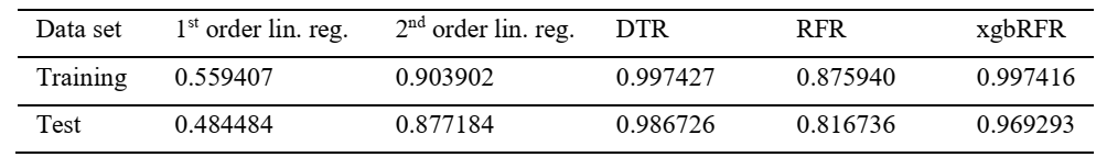
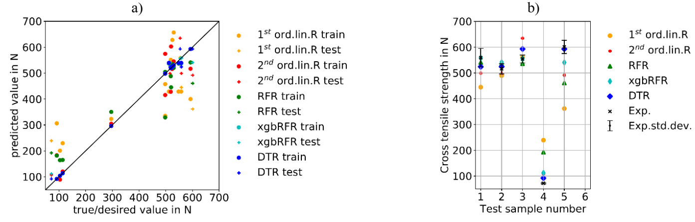Fig. 1. Prediction performance of employed regression models 1^st and 2^nd order linear regressions, decision tree regression (DTR), random forest regression (RFR) and XGBoosted RFR (xgbRFR): (a) Predicted vs true values of CTS in N (b) test sample predictions and experimental values (Exp.) with experimental standard deviations (Exp.std.dev.).

5.2 Model interpretations

     To provide an explanation on each model prediction, the feature importance for DTR, RFR, xgbRFR and 2^nd order linear regression is shown in Figure 2. The ascending features order is in accordance to their respective average impact on model output magnitude (mean of absolute SHAP values), i.e. feature importance. DTR represents the simplest model, as only five features are considered important, generating the highest determination coefficient R²; thus, exhibiting best prediction performance among all models. For xgbRFR, RFR and 2^nd order linear regression, the quadratic feature PD² is most important, respectively. For xgbRFR, eight features are denoted with means of absolute SHAP values above zero; therefore can be considered important. Whereas for RFR and 2^nd order linear regression, all nine features are important to some extend. There is also an increasing number of features considered relevant from DTR, to xgbRFR and to RFR because the forests are based on variations of randomly selected features used for the containing trees and more features are considered important, as they are inevitably composing the average, i.e. the output, of the forests.

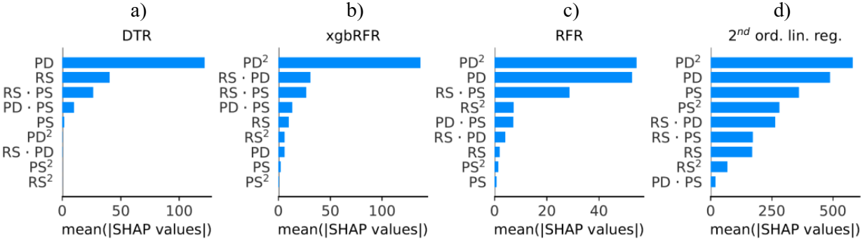
Fig. 2. SHAP feature importance of employed regression models: (a) Decision tree regression (DTR) (b), xg-boosted random forest (xgbRFR), (c) random forest (RFR), and (d) 2^nd order linear regression.

In Figure 3, the feature values (from low to high) are assigned to their impact on the model outputs. When comparing the tree-based models (a-c) to the 2^nd order linear regression (d), it can be seen that the former exhibit non-symmetric distributions of SHAP values in relation to the zero-axis, whereas the latter displays a symmetric distribution. On the one hand, feature values that are either very low or very high carry similar impact on the 2^nd order linear regression model output. On the other hand, whether a feature value is highest or lowest makes a difference on the impact on the tree-based models output.

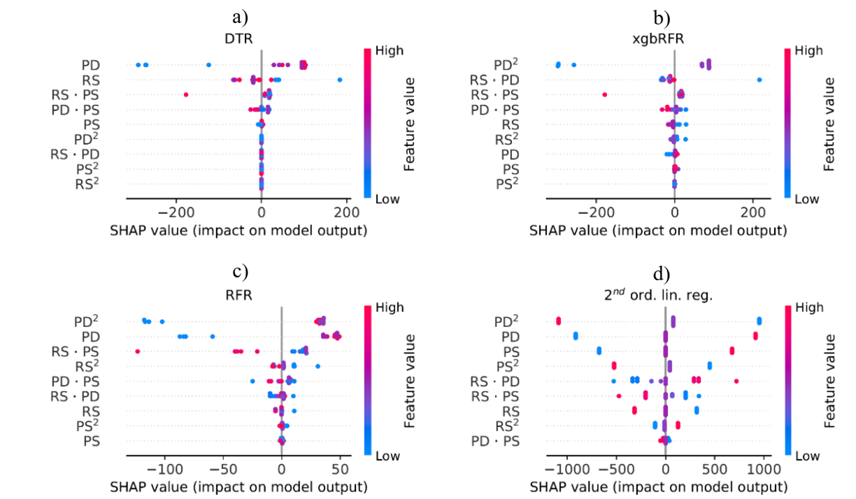Fig. 3. SHAP feature dependency of employed regression models: (a) Decision tree regression (DTR), (b) xg-boosted random forest (xgbRFR),  (c) random forest (RFR), and (d) 2^nd order linear regression.

     The detailed structure of the best-performing DTR and the corresponding specific decisions determined by the model to accurately predict CTS are illustrated in Figure 4. The initial decision of the DTR is based on the plunge depth PD being above or below 0.6 mm, which is equivalent to the sheet thickness. Furthermore, it can be inferred, which specific process parameter combinations lead to particular CTS, similar to results obtained from the response surface methodology in [14]. For example, setting PD above 0.6 mm and RS below 1875 min^-1, yields CTS values above 498 N. The number of leafs, i.e. number of final nodes, in the DTR corresponds to the number of different parameter sets in the Box-Behnken DoE. Since the MSE equates to zero in all single-sample leafs, most training samples were memorized by the trained DTR, reasoned by the extremely small training set size. As a result, a test prediction with a parameter combination unseen by the DTR during training is assigned the training sample output value which happens to be closest to the one of the test sample. Ultimately, application of a DTR leads to an improved R² in comparison to linear regression and can deliver another perspective on identified feature importance to predict CTS, which was previously hidden when only using linear models.

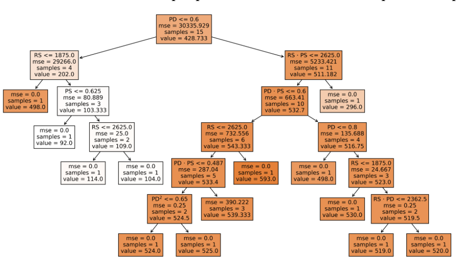Fig. 4. Decision tree regression (DTR) model for predicting CTS based on process parameters: Rotational speed (RS), plunge depth (PD) and plunge speed (PS).

6 Conclusion

     In conclusion, it was shown that the utilization of non-linear machine learning models to perform regression analysis can be beneficial with respect to achieving low prediction errors, especially in comparison to purely linear regression models. In case of this study, DTR was selected as the best model to predict CTS based on the Box-Behnken DoE data set used for training. Exploitation of such an explainable machine-learning algorithm provides additional understanding about the process and allow for inference on importance of process parameters and their values for prediction of mechanical properties with low prediction errors.

Acknowledgements

This work has been conducted within the scope of the European Project DAHLIAS (Development and Application of Hybrid Joining in Lightweight Integral Aircraft Structures). The DAHLIAS project is funded by European Union’s HORIZON 2020 framework program, Clean Sky 2 Joint Undertaking, and AIRFRAME ITD under grant agreement number 821081.